# basic imports
import numpy as np
import pandas as pd
import seaborn as sns
import matplotlib.pyplot as plt

# machine learning imports
from sklearn.model_selection import train_test_split
from sklearn.datasets import make_blobs
from sklearn.neighbors import KNeighborsClassifier
from sklearn.dummy import DummyClassifier
from sklearn.metrics import accuracy_score
from sklearn.metrics import confusion_matrix
from sklearn.metrics import ConfusionMatrixDisplayClassification Introduction
Like Regression, But Different
Objectives
In this note, we will discuss:
- the supervised learning classification task,
- the Bayes classifier,
- \(k\)-nearest neighbors for classification,
- classification metrics,
- and estimating conditional probabilities with a learned classification model.
Along the way, you should notice that except for the conditional probabilities, the process followed mirrors that of regression.
Python Setup
Notebook
The following Jupyter notebook contains some starter code that may be useful for following along with this note.
The Goal of Classification
Like regression, classification is a supervised learning task. However, while regression is concerned with predicting a numeric target variable, classification seeks to predict a categorical target variable.
To introduce classification, we simulate some data using the make_blobs function from the sklearn datasets module.
X, y = make_blobs(
    n_samples=800,
    n_features=2,
    centers=3,
    cluster_std=4.5,
    random_state=42,
)
y = y.astype("str")
The details of this code are not particularly important, however we should note that we have created 800 samples of two features (n_features=2) and that the response y has three categories (centers=3).
Now that we understand the importance of data splitting, we immediately train-test split this data.
X_train, X_test, y_train, y_test = train_test_split(
    X,
    y,
    test_size=0.20,
    random_state=42,
)
With the data split, let’s take a look at the train data.
| \(x_1\) | \(x_2\) | \(y\) |
|---|---|---|
| 2.12 | 3.67 | 1 |
| -1.11 | 15.65 | 0 |
| -4.83 | 2.86 | 2 |
| 11.41 | 5.92 | 1 |
| -6.73 | -10.34 | 2 |
| -2.81 | 3.56 | 0 |
| 11.81 | -0.33 | 1 |
| -8.00 | 0.35 | 2 |
| 5.07 | -0.11 | 1 |
| 3.37 | 9.11 | 0 |
As always, the tabular view of the data is not particularly informative. Instead, we create a scatterplot. To increase the effectiveness of the scatterplot, we use Seaborn’s jointplot to add density estimates for each category marginally for each feature variable.
Show Code for Plot
joint = sns.jointplot(
    x=X_train[:, 0],
    y=X_train[:, 1],
    hue=y_train,
    edgecolor="k",
    alpha=0.75,
    space=0,
)
joint.set_axis_labels(
    xlabel="$x_1$",
    ylabel="$x_2$",
)
joint.ax_joint.legend(
    loc="lower left",
)
plt.show()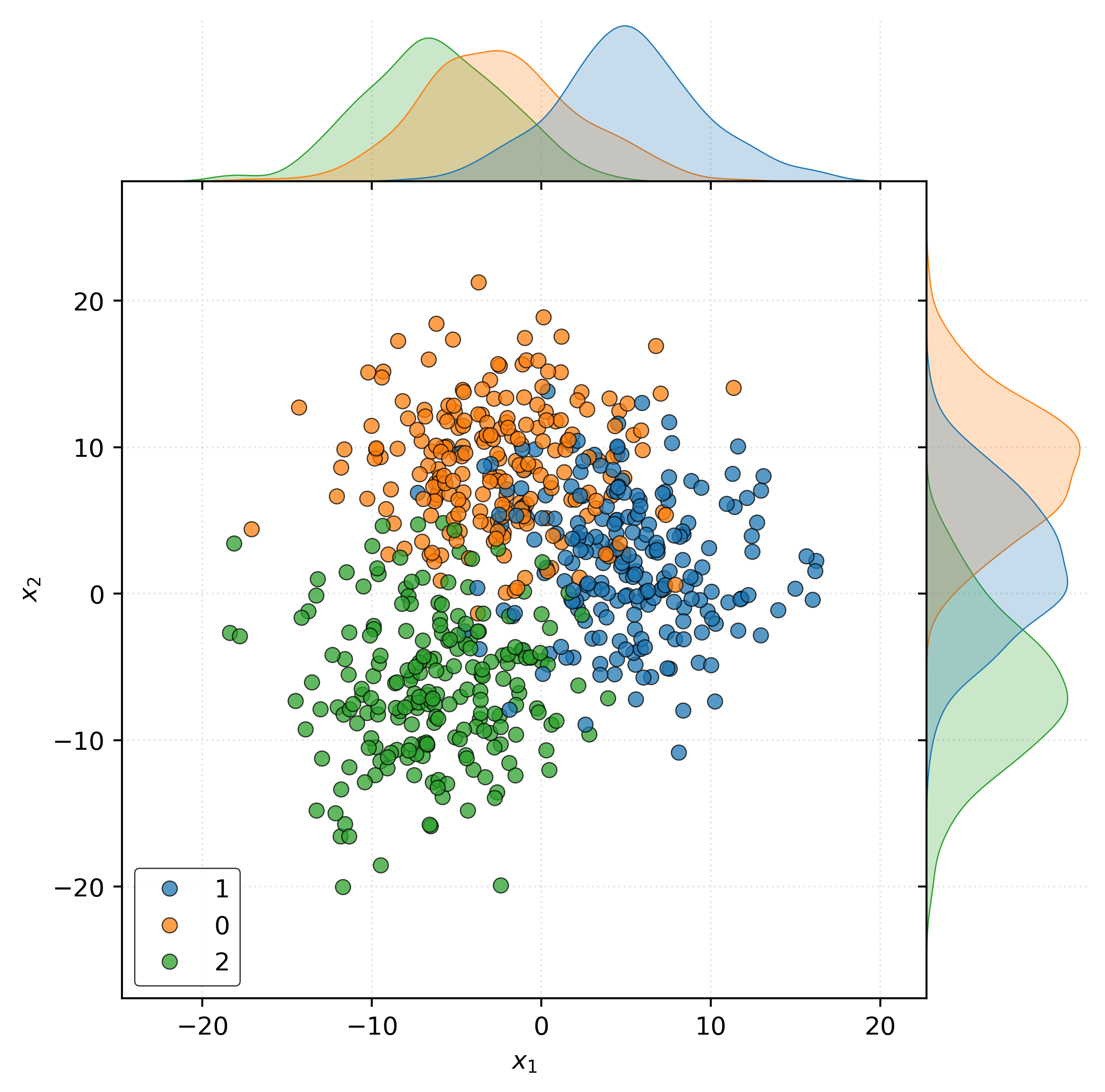
Consider new data at \(\pmb{x} = (x_1, x_2)\). The goal of classification is to predict the class label \(y\) for this new data point.
Specifically consider the following example when \(\pmb{x} = (-5, 5)\).
Show Code for Plot
joint = sns.jointplot(
    x=X_train[:, 0],
    y=X_train[:, 1],
    hue=y_train,
    edgecolor="k",
    alpha=0.75,
    space=0,
)
joint.set_axis_labels(
    xlabel="$x_1$",
    ylabel="$x_2$",
)
joint.ax_joint.legend(
    loc="lower left",
)
joint.ax_joint.plot(
    -5,
    5,
    marker="o",
    markersize=10,
    color="red",
)
plt.show()
The fundamental question that classification seeks to answer is: what is the probability that \(Y = g\) given \(\pmb{X} = \pmb{x}\)?
So, in this case, what is the probability that:
- \(Y = 0\) (blue) when \(\pmb{x} = (-5, 5)\)?
- \(Y = 1\) (orange) when \(\pmb{x} = (-5, 5)\)?
- \(Y = 2\) (green) when \(\pmb{x} = (-5, 5)\)?
With these questions answered, we can then make a prediction for the class label of \(\pmb{x} = (-5, 5)\). Simply predict the class label with the highest probability!
Unfortunately, we do not know the true conditional probabilities. So instead, we will fit a model that can be used to estimate these probabilities.
Bayes Classifier
The Bayes Classifier, \(C^B(x)\), is the classifier that minimizes the probability of misclassification, and thus is considered the optimal classifier. However, the Bayes Classifier cannot be used in practice as it requires knowledge of the true conditional probabilities. It is simply a useful concept for theoretical understanding of classification.
\[ p_g(\pmb{x}) = P\left[ Y = g \mid \pmb{X} = \pmb{x} \right] \]
\[ C^B(\pmb{x}) = \underset{g \in \{1, 2, \ldots G\}}{\text{argmax}} \ p_g(\pmb{x}) \]
The Bayes Classifier simply says “predict the class label with the highest conditional probability given feature values \(\pmb{x}\)”.
For the data in Figure 2, suppose we knew the following to be true:
- \(P[Y = 0 \mid \pmb{X} = (-5, 5)] = 0.70\)
- \(P[Y = 1 \mid \pmb{X} = (-5, 5)] = 0.20\)
- \(P[Y = 2 \mid \pmb{X} = (-5, 5)] = 0.10\)
Then in this case, the Bayes Classifier tells us to predict \(Y = 0\).
While a simple idea, it is the basis for theoretical understanding of classification.
Building a Classifier
Given that we cannot use the Bayes Classifier in practice, we will build a model that can be used to estimate the relevant conditional probabilities. With those estimated probabilities, we can then make predictions using the same rule as the Bayes Classifier, but with the estimated probabilities rather than known conditional probabilities.
\[ \hat{p}_g(\pmb{x}) = \hat{P}\left[ Y = g \mid \pmb{X} = \pmb{x} \right] \]
\[ \hat{C}(\pmb{x}) = \underset{g \in \{1, 2, \ldots G\}}{\text{argmax}} \ \hat{p}_g(\pmb{x}) \]
So in some sense, we use \(\hat{p}_g(\pmb{x})\) to estimate the true conditional probabilities \(p_g(\pmb{x})\). Then we create \(\hat{C}(\pmb{x})\) (using \(\hat{p}_g(\pmb{x})\)) as an estimate of the Bayes Classifier \(C^B(\pmb{x})\).
\(k\)-Nearest Neighbors
Our first model for classification will be the \(k\)-nearest neighbors classifier. Using \(k\)-nearest neighbors for classification is quite similar to \(k\)-nearest neighbors for regression.
After finding the \(k\)-nearest neighbors of \(\pmb{x}\), we will predict the class label of \(\pmb{x}\) as the class label that is most common among the \(k\)-nearest neighbors. More specifically, we can utilize the \(k\)-nearest neighbors to estimate the conditional probabilities. We will simply count the number of neighbors of each class label and divide by \(k\) to get the estimated probabilities!
\[ \hat{p}_g(\pmb{x}) = \hat{P}\left[ Y = g \mid \pmb{X} = \pmb{x} \right] = \frac{1}{k} \sum_{i \in \mathcal{N}_k(x)} I(y_i = g) \]
After estimating the conditional probabilities, we can then make a prediction for the class label of \(\pmb{x}\) that has the highest estimated conditional probability.
\[ \hat{C}(\pmb{x}) = \underset{g \in \{1, 2, \ldots G\}}{\text{argmax}} \hat{p}_g(\pmb{x}) \]
Like \(k\)-nearest neighbors for regression, \(k\)-nearest neighbors for classification requires specifying (or tuning) a value for \(k\).
Classification Metrics
There are many metrics to evaluate the performance of a classifier. We will detail a long list of them in the future. For introductory purposes, we will focus on two metrics: accuracy and misclassification.
\[ \text{Accuracy}(y, \hat{y}) = \frac{1}{n} \sum_{i=1}^{n} I(y_i = \hat{y}_i) \]
\[ I(y_i = \hat{y}_i) = \begin{cases} 1 & \text{if } y_i = \hat{y}_i \\ 0 & \text{otherwise} \end{cases} \]
The accuracy is simply the proportion of correct predictions made by the classifier. We will see that accuracy is in many ways the default metric for classification, especially within sklearn. Like regression metrics, sklearn provides functions to calculate classification metrics, including the accuracy_score function.
Note that unlike RMSE for regression, which we want to minimize, accuracy is a metric that we want to maximize. The classification error, or misclassification rate, is simply the proportion of incorrect predictions made by the classifier. So while these two metrics are related, and essentially measure the same thing, it can sometimes be useful to consider errors instead of correct predictions.
\[ \text{Misclassification}(y, \hat{y}) = \frac{1}{n} \sum_{i=1}^{n} I(y_i \neq \hat{y}_i) \]
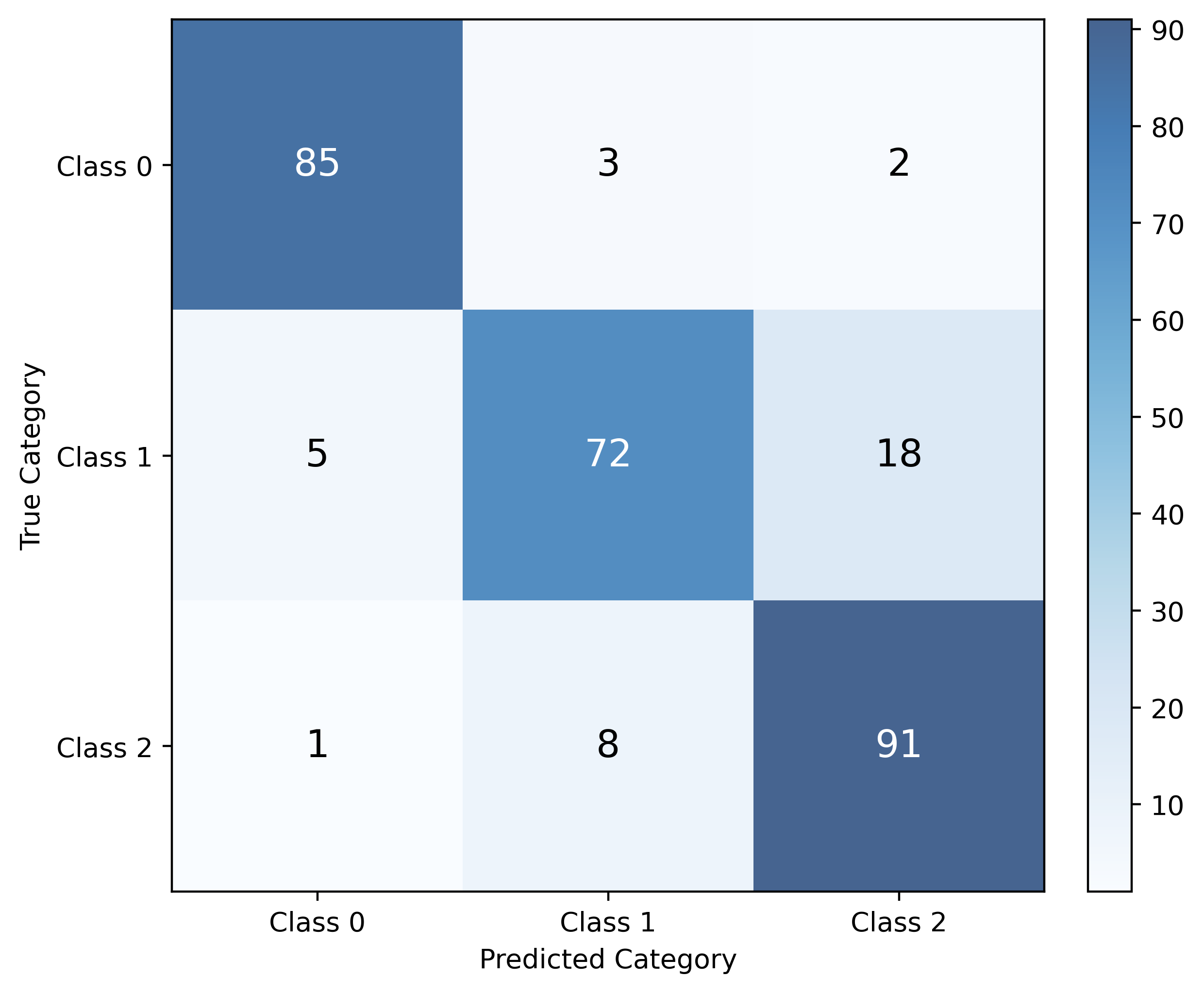
Confusion Matrix
While accuracy tells us the overall proportion of correct predictions, it doesn’t reveal where our classifier makes mistakes. A confusion matrix provides a more detailed view of classifier performance by showing the counts of actual versus predicted classifications for each class.
For a classification problem with \(G\) categories (classes), the confusion matrix is a \(G \times G\) table where:
- Rows represent the true (actual) categories
- Columns represent the predicted categories
- Each cell \((i,j)\) contains the count of observations that were actually class \(i\) but predicted as class \(j\)
The diagonal elements represent correct predictions, while off-diagonal elements represent misclassifications. This detailed breakdown helps us understand not just how often our classifier is wrong, but specifically which classes it confuses with each other.
\(k\)-Nearest Neighbors Classifier with sklearn
Now we’ll use sklearn’s KNeighborsClassifier to build a classification model and fit it to the simulated data. The workflow follows the same pattern as other sklearn estimators: initialize the model, fit to the data, and predict on new data.
First, we create a KNN classifier object, specifying a particular number of neighbors, \(k\), to use:
knn = KNeighborsClassifier(n_neighbors=7)Next, we use the .fit() method to fit the classifier to the training data:
_ = knn.fit(X_train, y_train)With the model fit, we can make predictions using the .predict() method:
print(knn.predict(X_test[:5]))['0' '1' '1' '2' '0']So far, the only difference between classifier and regression is the use of KNeighborsClassifier instead of KNeighborsRegressor.
With KNeighborsClassifier, in addition to .fit() and .predict(), we can also use the .predict_proba() method to obtain estimated conditional probabilities:
print(knn.predict_proba(X_test[:5]))[[0.7143 0.2857 0. ]
[0. 1. 0. ]
[0. 1. 0. ]
[0. 0. 1. ]
[0.7143 0.2857 0. ]]This returns the estimated conditional probability of each class given each observation (in the test data).
For example, consider the first observation in the test set:
X_test[:1]array([[-0.2249, 6.7124]])The first row of the output above corresponds to the estimated conditional probabilities for this observation.
print(knn.predict_proba(X_test[:1]))[[0.7143 0.2857 0. ]]Writing this output more mathematically, we have:
- \(\hat{P}[Y = 0 \mid \pmb{X} = (-0.22, 6.71)] = 0.71\)
- \(\hat{P}[Y = 1 \mid \pmb{X} = (-0.22, 6.71)] = 0.29\)
- \(\hat{P}[Y = 2 \mid \pmb{X} = (-0.22, 6.71)] = 0.00\)
To demonstrate calculating test accuracy for this classifier, we make predictions on the entire test set then use the accuracy_score() function to calculate test accuracy:
y_pred = knn.predict(X_test)
accuracy_score(y_test, y_pred)0.88125We can examine the confusion matrix to see where misclassifications occur:
print(confusion_matrix(y_test, y_pred))[[49 3 1]
[ 9 39 3]
[ 1 2 53]]To “visualize” the confusion matrix, we can use sklearn’s ConfusionMatrixDisplay (specifically the .from_predictions() method) to create a visual confusion matrix:
fig, ax = plt.subplots(figsize=(6, 5))
ConfusionMatrixDisplay.from_predictions(
    y_test,
    y_pred,
    ax=ax,
    im_kw={"cmap": "Blues", "alpha": 0.75}
)
ax.set_xlabel("Predicted Category")
ax.set_ylabel("True Category")
ax.grid(False)
plt.show()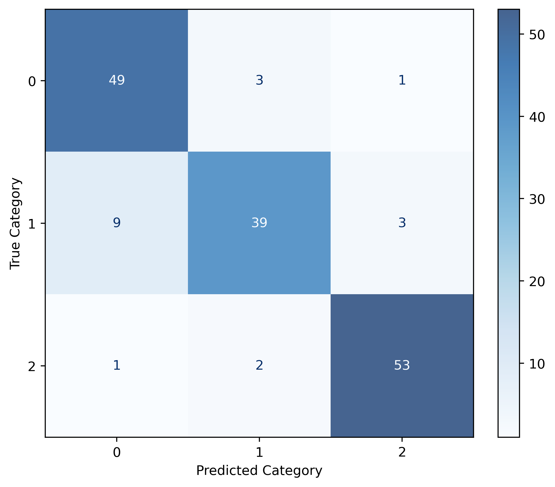
Example: Tuning a \(k\)-Nearest Neighbors Classifier
Like we did for regression, let’s tune a KNN model for classification First, we split our train data into (validation) train and validation sets:
X_vtrain, X_validation, y_vtrain, y_validation = train_test_split(
    X_train,
    y_train,
    test_size=0.20,
    random_state=42,
)
We’ll evaluate a range of \(k\) values to find the optimal choice. Here, we’ll consider values from 1 to 501, stepping by 10:
k_values = range(1, 501, 10)
train_accuracies = []
validation_accuracies = []
For each candidate \(k\) value, we fit the model to the (validation) train data and evaluate on both the train and validation sets:
for k in k_values:
    knn = KNeighborsClassifier(n_neighbors=k)
    knn.fit(X_vtrain, y_vtrain)
    y_pred_train = knn.predict(X_vtrain)
    y_pred_validation = knn.predict(X_validation)
    train_accuracy = accuracy_score(y_vtrain, y_pred_train)
    validation_accuracy = accuracy_score(y_validation, y_pred_validation)
    train_accuracies.append(train_accuracy)
    validation_accuracies.append(validation_accuracy)
We select the \(k\) value that achieves the largest validation accuracy:
best_k = k_values[np.argmax(validation_accuracies)]
print(f"Best k: {best_k}")
print(f"Validation Accuracy: {max(validation_accuracies):.2f}")
Best k: 361
Validation Accuracy: 0.86For a visualization of these results, we’ll convert accuracies to error rates and plot them:
validation_error = 1 - np.array(validation_accuracies)
train_error = 1 - np.array(train_accuracies)
Show Code for Plot
fig, ax = plt.subplots()
ax.plot(
    k_values,
    train_error,
    label="Train Error",
    marker="o",
    markeredgecolor="black",
    markerfacecolor="tab:gray",
    markersize=3,
    lw=1,
)
ax.plot(
    k_values,
    validation_error,
    label="Validation Error",
    marker="o",
    markeredgecolor="black",
    markerfacecolor="tab:gray",
    markersize=3,
    lw=1,
)

ax.set_xlabel("k (Number of Neighbors)")
ax.set_ylabel("Error")
ax.invert_xaxis()
ax.legend()
plt.show()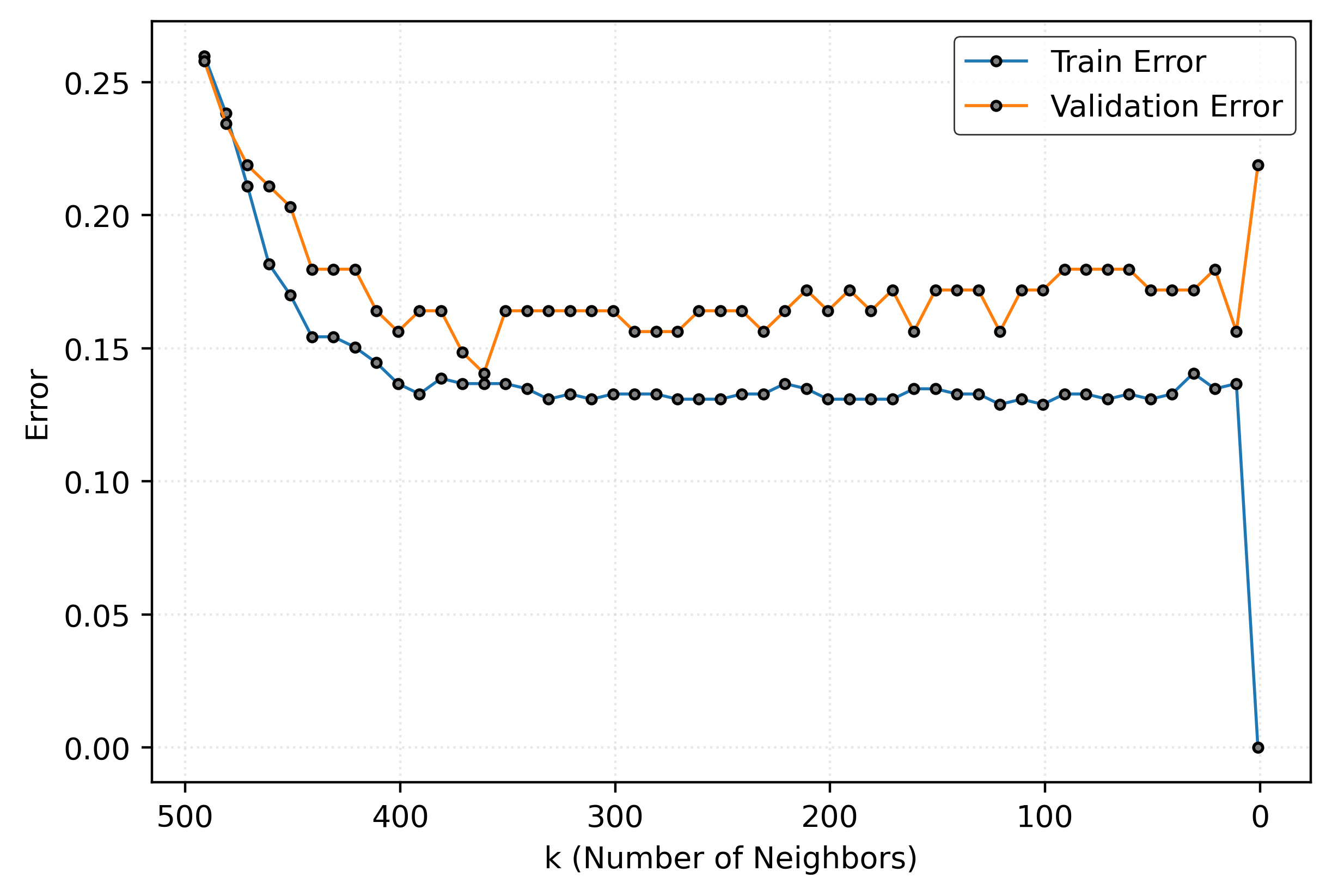
Figure 5 shows how model performance varies with \(k\). At very low \(k\) values, the model performs perfectly on training data but poorly on validation data. At very high \(k\) values, both training and validation performance suffer. The optimal \(k\) balances these extremes.
Let’s examine the class distribution in our validation set to understand our baseline performance:
proportions = pd.Series(y_validation).value_counts(normalize=True)
print(proportions)
1 0.37
0 0.32
2 0.31
Name: proportion, dtype: float64This shows the proportion of each class. A “dummy” classifier that always predicts the most common class would achieve an accuracy equal to the largest proportion above.
Finally, we refit our tuned model to the (full) train set and evaluate on the test data:
knn = KNeighborsClassifier(n_neighbors=best_k)
knn.fit(X_train, y_train)
y_pred_test = knn.predict(X_test)
test_accuracy = accuracy_score(y_test, y_pred_test)
print(f"Test Accuracy: {test_accuracy:.2f}")
Test Accuracy: 0.88This test accuracy provides our final, unbiased estimate of how well our tuned KNN classifier will perform on new, unseen data.
We can also examine the estimated conditional probabilities for some test observations:
print(knn.predict_proba(X_test)[:10])[[0.5319 0.3934 0.0748]
[0.2244 0.5651 0.2105]
[0.2216 0.5762 0.2022]
[0.205 0.2133 0.5817]
[0.5568 0.338 0.1053]
[0.5762 0.3906 0.0332]
[0.5319 0.2022 0.2659]
[0.2742 0.1468 0.5789]
[0.1274 0.4404 0.4321]
[0.5817 0.3241 0.0942]]Let’s compare these probabilities with the actual test labels:
print(y_test[:10])['1' '1' '1' '2' '0' '0' '0' '2' '1' '0']And the predicted labels:
print(y_pred_test[:10])['0' '1' '1' '2' '0' '0' '0' '2' '1' '0']For a clearer comparison, we can create a summary table showing actual labels, predictions, and probabilities:
results_df = pd.DataFrame(
    {
        "Actual": y_test[:10],
        "Predicted": y_pred_test[:10],

    }
)
prob_df = pd.DataFrame(knn.predict_proba(X_test)[:10])
prob_df.columns = [f"prob_{i}" for i in knn.classes_]
results_df = pd.concat([results_df, prob_df], axis=1)
print(results_df)
Actual Predicted prob_0 prob_1 prob_2
0 1 0 0.53 0.39 0.07
1 1 1 0.22 0.57 0.21
2 1 1 0.22 0.58 0.20
3 2 2 0.20 0.21 0.58
4 0 0 0.56 0.34 0.11
5 0 0 0.58 0.39 0.03
6 0 0 0.53 0.20 0.27
7 2 2 0.27 0.15 0.58
8 1 1 0.13 0.44 0.43
9 0 0 0.58 0.32 0.09This table helps us understand the model’s confidence in its predictions and identify cases where the model might be uncertain.