# basic imports
import numpy as np
import pandas as pd
import seaborn as sns
import matplotlib.pyplot as plt

# machine learning imports
from sklearn.model_selection import train_test_split
from sklearn.neighbors import KNeighborsClassifier
from sklearn.metrics import accuracy_score

# preprocessing imports
from sklearn.preprocessing import StandardScaler
from sklearn.preprocessing import OneHotEncoder
from sklearn.impute import SimpleImputer
from sklearn.compose import make_column_transformer
from sklearn.pipeline import make_pipeline

# data imports
from palmerpenguins import load_penguinsPreprocessing
Modeling Heterogeneous and Missing Data
Objectives
In this note, we will cover various preprocessing techniques and their applications, including:
- Numeric Scaling: Standardizing numeric features to have a mean of 0 and a standard deviation of 1.
- Categorical Encoding: Converting categorical features into (multiple) numeric features using one-hot encoding.
- Imputation: Handling missing data by replacing missing values.
- Pipelines: Combining preprocessing steps (with a column transformer) and machine learning models for seamless application.
To summarize these techniques, we will demonstrate their applications using the Palmer Penguins dataset.
Python Setup
Notebook
The following Jupyter notebook contains some starter code that may be useful for following along with this note.
Motivation
The following function can be used to simulate data with mixed types (numeric and categorical) and missing data.
def simulate_mixed_data(n_samples=10, missing_rate=0.2, random_state=42):

    # set random seed for reproducibility
    np.random.seed(random_state)

    # create DataFrame with mixed data types
    df = pd.DataFrame(
        {
            "num_big": np.random.normal(1000, 100, n_samples),
            "num_small": np.random.normal(0, 1, n_samples),
            "cat_str": np.random.choice(["A", "B", "C"], n_samples),
            "cat_num": np.random.choice([0, 1], n_samples),
            "target": np.random.choice([0, 1], n_samples),
        }
    )

    # add missing values to feature columns only
    for col in df.columns[:-1]:
        missing_mask = np.random.random(n_samples) < missing_rate
        df.loc[missing_mask, col] = np.nan

    # return the DataFrame with mixed feature types
    return df
Why do we need to preprocess data? There are two main reasons:
- Preprocessing can be necessary to make modeling possible.
- Preprocessing can be used to improve model performance.
df = simulate_mixed_data()
df| num_big | num_small | cat_str | cat_num | target | |
|---|---|---|---|---|---|
| 0 | 1,049.67 | -0.46 | B | 0.00 | 1 |
| 1 | 986.17 | -0.47 | B | 0.00 | 0 |
| 2 | NaN | 0.24 | C | NaN | 1 |
| 3 | 1,152.30 | -1.91 | B | NaN | 0 |
| 4 | NaN | -1.72 | C | 1.00 | 1 |
| 5 | 976.59 | -0.56 | C | 1.00 | 1 |
| 6 | 1,157.92 | -1.01 | A | 0.00 | 1 |
| 7 | 1,076.74 | 0.31 | NaN | 1.00 | 0 |
| 8 | 953.05 | -0.91 | NaN | 1.00 | 1 |
| 9 | NaN | -1.41 | C | 1.00 | 0 |
df.dtypesnum_big float64
num_small float64
cat_str object
cat_num float64
target int64
dtype: objectConsider this data frame created using the function above. We have two numeric features. We also have two categorical features, one that is currently encoded as strings. Many of the feature variables contain missing data.
Now consider modeling this data with \(k\)-nearest neighbors. What is the distance between the features of the first and third samples?
   num_big  num_small cat_str  cat_num
0 1,049.67      -0.46       B     0.00
2      NaN       0.24       C      NaN
KNN, like many machine learning methods require all input features to be numeric and free of missing data. Until we have dealt with any missing data, we cannot fit the model. Additionally, something will need to be done to the cat_str variable, as we cannot include values like “B” in distance calculations. Transformations that remove these issues make modeling possible.
Also notice that the two numeric features are on wildly different scales. We could consider scaling them, thus putting them on the same scale. This is an example of a transformation that could improve model performance. But keep in mind, it isn’t a guarantee, but it could help.
Numeric Scaling
When features exist on vastly different scales, algorithms that rely on distance calculations can be dominated by the feature with the largest scale. Let’s address this by applying standardization (also called z-score normalization) to our numeric features.
First, let’s isolate the numeric columns in the data frame we created.
df_numeric = df[["num_big", "num_small"]]
df_numeric| num_big | num_small | |
|---|---|---|
| 0 | 1,049.67 | -0.46 |
| 1 | 986.17 | -0.47 |
| 2 | NaN | 0.24 |
| 3 | 1,152.30 | -1.91 |
| 4 | NaN | -1.72 |
| 5 | 976.59 | -0.56 |
| 6 | 1,157.92 | -1.01 |
| 7 | 1,076.74 | 0.31 |
| 8 | 953.05 | -0.91 |
| 9 | NaN | -1.41 |
We’ll use StandardScaler from sklearn, which as the the suggests, can be used to standardize variables.
While not a class for a model like KNeighborsClassifier, the StandardScaler has a similar usage patten: create, fit, then transform (rather than predict).
So, we first create a StandardScaler object.
standard_scaler = StandardScaler()The standardization transformation applied to each column is
\[ x_j^{\prime} = \frac{x_j - \bar{x}_j}{s_{x_j}}, \]
where \(x_j^{\prime}\) is the standardized value, \(\bar{x}_j\) is the mean of feature \(j\), and \(s_{x_j}\) is the standard deviation of feature \(j\). This transformation centers each feature around zero and scales it to have unit variance.
Next, we fit the scaler to learn the mean and standard deviation of some input data, using the .fit() method.
_ = standard_scaler.fit(df_numeric)Let’s examine what the scaler learned about our data’s distribution:
print(f"Initial Column Means: {standard_scaler.mean_}")
print(f"Initial Column Standard Deviations: {standard_scaler.scale_}")
Initial Column Means: [ 1.0504e+03 -7.9066e-01]
Initial Column Standard Deviations: [77.1729 0.7166]Now we can transform data using these learned parameters:
print(standard_scaler.transform(df_numeric))[[-0.0088 0.4567]
[-0.8316 0.4535]
[ nan 1.4411]
[ 1.3211 -1.5667]
[ nan -1.3038]
[-0.9558 0.3187]
[ 1.3939 -0.3101]
[ 0.342 1.5419]
[-1.2608 -0.1638]
[ nan -0.8675]]To verify our transformation worked as expected, let’s calculate the means and standard deviations of the transformed data:
transformed_numeric_array = standard_scaler.transform(df_numeric)
transformed_col_mean = np.nanmean(transformed_numeric_array, axis=0)
transformed_col_std = np.nanstd(transformed_numeric_array, axis=0)

print(f"Transformed Column Means: {transformed_col_mean}")
print(f"Transformed Column Standard Deviations: {transformed_col_std}")
Transformed Column Means: [ 4.7581e-16 -4.4409e-17]
Transformed Column Standard Deviations: [1. 1.]Notice that after standardization, both features now have means essentially equal to zero and standard deviations equal to one. This puts both features on the same scale, ensuring that neither will dominate distance calculations in our machine learning algorithms.
Impact of Scaling
Why does scaling impact KNN? Recall how KNN makes predictions: it finds the \(k\) nearest neighbors based on distance calculations. When features have vastly different scales, the feature with the larger scale will dominate the distance computation, effectively making the smaller-scale features irrelevant.
Consider a scenario where one feature represents income (ranging from $30,000 to $100,000) and another represents age (ranging from 20 to 65). In the raw scale, a difference of $1,000 in income will have a much larger impact on the distance calculation than a difference of 10 years in age, even though both might be equally important for the prediction task.
Let’s visualize this effect.
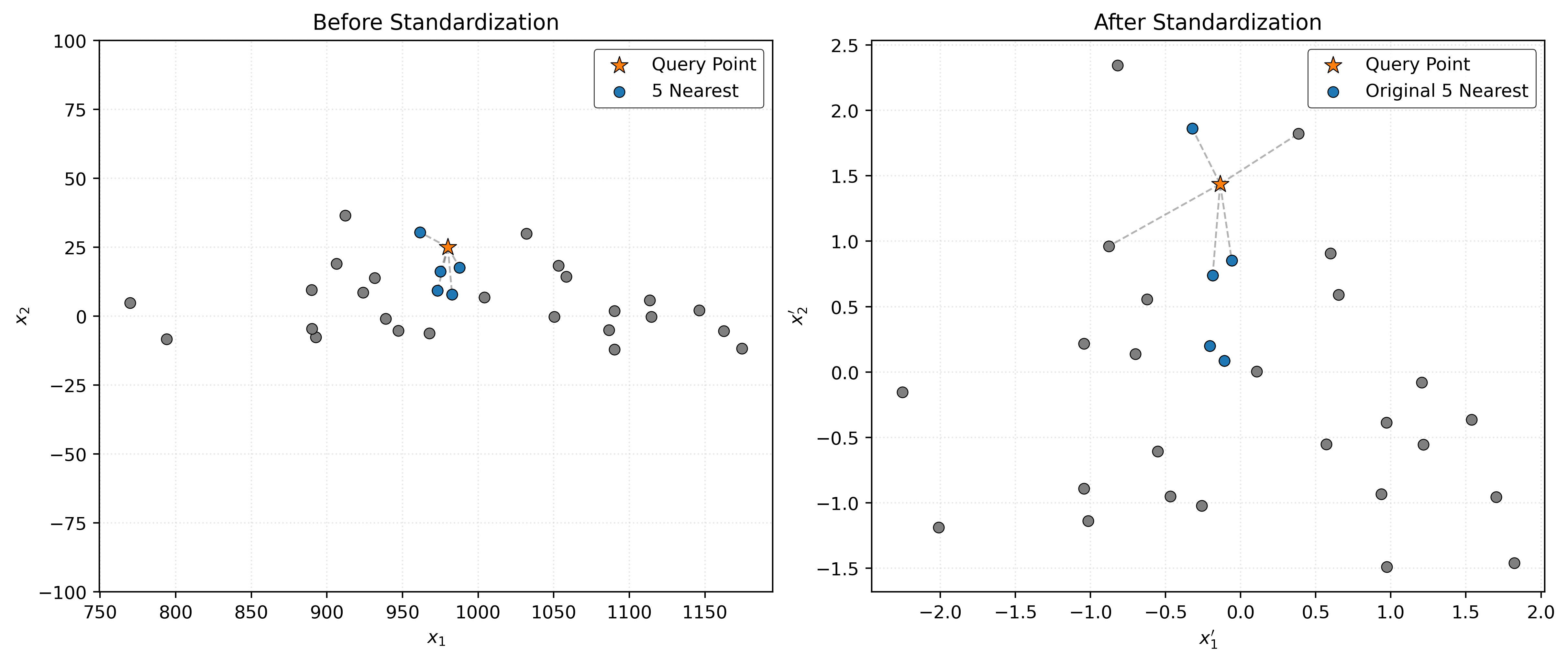
In Figure 1, we see a dramatic difference between the two scenarios. In the left panel (before standardization), the 5 nearest neighbors to our query point (orange star) are all clustered tightly along the \(x_1\) dimension because the scale difference means that small variations in \(x_1\) (around 1000) completely overwhelm much larger proportional variations in \(x_2\) (around 5).
After standardization (right panel), both dimensions contribute equally to the distance calculation. Now the 5 nearest neighbors are distributed more evenly around the query point in both dimensions, giving us a more balanced and intuitive notion of “nearness.”
This visualization demonstrates why scaling is often essential for distance-based algorithms like KNN. Without proper scaling, these algorithms can produce misleading results where one feature inadvertently dominates the prediction process.
Categorical Encodings
While scaling can addresses issues with numeric features, we face a different challenge with categorical variables. Most machine learning algorithms expect numeric inputs, but categories like A, B, C have no inherent mathematical meaning. We can’t simply convert A to 1, B to 2, and C to 3, because this would imply that B is “twice as much” as A, and C is “three times” as much, which is meaningless for categorical data.
Our simulated dataset contains two types of categorical features.
df_categorical = df[["cat_str", "cat_num"]]
df_categorical| cat_str | cat_num | |
|---|---|---|
| 0 | B | 0.00 |
| 1 | B | 0.00 |
| 2 | C | NaN |
| 3 | B | NaN |
| 4 | C | 1.00 |
| 5 | C | 1.00 |
| 6 | A | 0.00 |
| 7 | NaN | 1.00 |
| 8 | NaN | 1.00 |
| 9 | C | 1.00 |
Notice that we have both string categories (A, B, C) and numeric categories (0, 1). Even though cat_num uses numbers, these are still categorical. The values 0 and 1 represent distinct categories (in this case), not quantities where 1 is “more” than 0 in any meaningful sense.
One-Hot Encoding
The most common solution for categorical variables is one-hot encoding. This approach creates a separate binary column for each category, where 1 indicates the presence of that category and 0 indicates its absence.
Let’s see how OneHotEncoder from sklearn transforms categorical data.
Like StandardScaler we first create an encoder, then use .fit() to learn the encoding, then use .transform() to apply the learned transformation to data.
one_hot_encoder = OneHotEncoder()
_ = one_hot_encoder.fit(df_categorical)
print(one_hot_encoder.transform(df_categorical).todense())
[[0. 1. 0. 0. 1. 0. 0.]
[0. 1. 0. 0. 1. 0. 0.]
[0. 0. 1. 0. 0. 0. 1.]
[0. 1. 0. 0. 0. 0. 1.]
[0. 0. 1. 0. 0. 1. 0.]
[0. 0. 1. 0. 0. 1. 0.]
[1. 0. 0. 0. 1. 0. 0.]
[0. 0. 0. 1. 0. 1. 0.]
[0. 0. 0. 1. 0. 1. 0.]
[0. 0. 1. 0. 0. 1. 0.]]The output shows a binary matrix, but it’s hard to interpret without column labels. Also, by default, this transformation uses a sparse representation, but to make it human-readable, we use the .todense() to reveal the dense representation. Let’s first examine what categories the encoder discovered.
one_hot_encoder.categories_[array(['A', 'B', 'C', nan], dtype=object), array([ 0., 1., nan])]The encoder found 4 categories for cat_str (A, B, C, nan) and 3 categories for cat_num (0, 1, nan). By default, OneHotEncoder() views any missing data as a category.1 Now let’s see the encoded data with informative column names.
print(
    pd.DataFrame(
        one_hot_encoder.transform(df_categorical).todense(),
        columns=one_hot_encoder.get_feature_names_out(),
    )
)
cat_str_A cat_str_B cat_str_C cat_str_nan cat_num_0.0 cat_num_1.0 \
0 0.00 1.00 0.00 0.00 1.00 0.00
1 0.00 1.00 0.00 0.00 1.00 0.00
2 0.00 0.00 1.00 0.00 0.00 0.00
3 0.00 1.00 0.00 0.00 0.00 0.00
4 0.00 0.00 1.00 0.00 0.00 1.00
5 0.00 0.00 1.00 0.00 0.00 1.00
6 1.00 0.00 0.00 0.00 1.00 0.00
7 0.00 0.00 0.00 1.00 0.00 1.00
8 0.00 0.00 0.00 1.00 0.00 1.00
9 0.00 0.00 1.00 0.00 0.00 1.00
cat_num_nan
0 0.00
1 0.00
2 1.00
3 1.00
4 0.00
5 0.00
6 0.00
7 0.00
8 0.00
9 0.00 Each original categorical column has been expanded into multiple binary columns. For example, if the original cat_str value was A, then cat_str_A becomes 1 and cat_str_B and cat_str_C become 0.
The transformation is reversible. We can recover the original categorical using the .inverse_transform() method.
one_hot_encoder.inverse_transform(one_hot_encoder.transform(df_categorical))array([['B', 0.0],
['B', 0.0],
['C', nan],
['B', nan],
['C', 1.0],
['C', 1.0],
['A', 0.0],
[nan, 1.0],
[nan, 1.0],
['C', 1.0]], dtype=object)This gives us back our original categorical data, confirming that no information was lost in the encoding process.
Dummy Encoding
One-hot encoding creates one column per category, but this can lead to a problem called exact collinearity. Notice that if we know the values of any \(c - 1\) columns in a one-hot encoded feature, we can perfectly predict the \(c\)th column. For example, assuming no missing data, if cat_str_A is 0 and cat_str_B is 0, then we know cat_str_C must be 1.
Dummy encoding addresses this by dropping one category column, keeping only \(c - 1\) columns for \(c\) categories. The dropped category becomes the “reference” category that’s implied when all other columns are 0.
dummy_encoder = OneHotEncoder(drop="first")
_ = dummy_encoder.fit(df_categorical)
print(dummy_encoder.transform(df_categorical).todense())
[[1. 0. 0. 0. 0.]
[1. 0. 0. 0. 0.]
[0. 1. 0. 0. 1.]
[1. 0. 0. 0. 1.]
[0. 1. 0. 1. 0.]
[0. 1. 0. 1. 0.]
[0. 0. 0. 0. 0.]
[0. 0. 1. 1. 0.]
[0. 0. 1. 1. 0.]
[0. 1. 0. 1. 0.]]Let’s see this with informative column names to understand what was dropped:
print(
    pd.DataFrame(
        dummy_encoder.transform(df_categorical).todense(),
        columns=dummy_encoder.get_feature_names_out(),
    )
)
cat_str_B cat_str_C cat_str_nan cat_num_1.0 cat_num_nan
0 1.00 0.00 0.00 0.00 0.00
1 1.00 0.00 0.00 0.00 0.00
2 0.00 1.00 0.00 0.00 1.00
3 1.00 0.00 0.00 0.00 1.00
4 0.00 1.00 0.00 1.00 0.00
5 0.00 1.00 0.00 1.00 0.00
6 0.00 0.00 0.00 0.00 0.00
7 0.00 0.00 1.00 1.00 0.00
8 0.00 0.00 1.00 1.00 0.00
9 0.00 1.00 0.00 1.00 0.00Notice that cat_str_A and cat_num_0.0 have been dropped. Now when all remaining columns are 0, it implicitly means the observation belongs to the reference category (A for cat_str, 0 for cat_num). This avoids exact collinearity while preserving all the categorical information.
Some methods, like KNN, are not impacted by exact collinearity. Other methods that we will see later, like linear regression, may act strange or be completely broken in the presence of exact collinearity.
Missing Data and Imputation
Numeric Features
simple_imputer = SimpleImputer(strategy="median")
_ = simple_imputer.fit(df_numeric)
print(simple_imputer.transform(df_numeric))
[[ 1.0497e+03 -4.6342e-01]
[ 9.8617e+02 -4.6573e-01]
[ 1.0497e+03 2.4196e-01]
[ 1.1523e+03 -1.9133e+00]
[ 1.0497e+03 -1.7249e+00]
[ 9.7659e+02 -5.6229e-01]
[ 1.1579e+03 -1.0128e+00]
[ 1.0767e+03 3.1425e-01]
[ 9.5305e+02 -9.0802e-01]
[ 1.0497e+03 -1.4123e+00]]Categorical Features
simple_imputer = SimpleImputer(strategy="most_frequent")
_ = simple_imputer.fit(df_categorical)
print(simple_imputer.transform(df_categorical))
[['B' 0.0]
['B' 0.0]
['C' 1.0]
['B' 1.0]
['C' 1.0]
['C' 1.0]
['A' 0.0]
['C' 1.0]
['C' 1.0]
['C' 1.0]]Pipelines and Column Transformers
df_sim = simulate_mixed_data(n_samples=500, missing_rate=0.1, random_state=42)df_train, df_test = train_test_split(df_sim, test_size=0.20, random_state=42)numeric_features = ["num_big", "num_small"]
categorical_features = ["cat_str", "cat_num"]
features = numeric_features + categorical_features
target = "target"X_train = df_train[features]
y_train = df_train[target]X_test = df_test[features]
y_test = df_test[target]numeric_transformer = make_pipeline(
SimpleImputer(strategy="median"),
StandardScaler(),
)categorical_transformer = make_pipeline(
SimpleImputer(strategy="most_frequent"),
OneHotEncoder(),
)preprocessor = make_column_transformer(
(numeric_transformer, numeric_features),
(categorical_transformer, categorical_features),
remainder="drop",
)preprocessor.fit(X_train)ColumnTransformer(transformers=[('pipeline-1',
Pipeline(steps=[('simpleimputer',
SimpleImputer(strategy='median')),
('standardscaler',
StandardScaler())]),
['num_big', 'num_small']),
('pipeline-2',
Pipeline(steps=[('simpleimputer',
SimpleImputer(strategy='most_frequent')),
('onehotencoder',
OneHotEncoder())]),
['cat_str', 'cat_num'])])In a Jupyter environment, please rerun this cell to show the HTML representation or trust the notebook. On GitHub, the HTML representation is unable to render, please try loading this page with nbviewer.org.
Parameters
| transformers | [('pipeline-1', ...), ('pipeline-2', ...)] | |
| remainder | 'drop' | |
| sparse_threshold | 0.3 | |
| n_jobs | None | |
| transformer_weights | None | |
| verbose | False | |
| verbose_feature_names_out | True | |
| force_int_remainder_cols | 'deprecated' |
['num_big', 'num_small']
Parameters
| missing_values | nan | |
| strategy | 'median' | |
| fill_value | None | |
| copy | True | |
| add_indicator | False | |
| keep_empty_features | False |
Parameters
| copy | True | |
| with_mean | True | |
| with_std | True |
['cat_str', 'cat_num']
Parameters
| missing_values | nan | |
| strategy | 'most_frequent' | |
| fill_value | None | |
| copy | True | |
| add_indicator | False | |
| keep_empty_features | False |
Parameters
| categories | 'auto' | |
| drop | None | |
| sparse_output | True | |
| dtype | <class 'numpy.float64'> | |
| handle_unknown | 'error' | |
| min_frequency | None | |
| max_categories | None | |
| feature_name_combiner | 'concat' |
print(preprocessor.transform(X_train))[[ 0.4214 -1.566 0. ... 0. 1. 0. ]
[ 0.7591 -0.0225 1. ... 0. 1. 0. ]
[-1.5424 0.8585 0. ... 1. 0. 1. ]
...
[-0.7926 -0.0225 1. ... 0. 0. 1. ]
[ 0.0638 -0.5497 0. ... 0. 0. 1. ]
[-0.3866 0.9913 0. ... 0. 1. 0. ]]knn_pipeline = make_pipeline(
preprocessor,
KNeighborsClassifier(n_neighbors=5),
)knn_pipeline.fit(X_train, y_train)Pipeline(steps=[('columntransformer',
ColumnTransformer(transformers=[('pipeline-1',
Pipeline(steps=[('simpleimputer',
SimpleImputer(strategy='median')),
('standardscaler',
StandardScaler())]),
['num_big', 'num_small']),
('pipeline-2',
Pipeline(steps=[('simpleimputer',
SimpleImputer(strategy='most_frequent')),
('onehotencoder',
OneHotEncoder())]),
['cat_str', 'cat_num'])])),
('kneighborsclassifier', KNeighborsClassifier())])In a Jupyter environment, please rerun this cell to show the HTML representation or trust the notebook. On GitHub, the HTML representation is unable to render, please try loading this page with nbviewer.org.
Parameters
| steps | [('columntransformer', ...), ('kneighborsclassifier', ...)] | |
| transform_input | None | |
| memory | None | |
| verbose | False |
Parameters
| transformers | [('pipeline-1', ...), ('pipeline-2', ...)] | |
| remainder | 'drop' | |
| sparse_threshold | 0.3 | |
| n_jobs | None | |
| transformer_weights | None | |
| verbose | False | |
| verbose_feature_names_out | True | |
| force_int_remainder_cols | 'deprecated' |
['num_big', 'num_small']
Parameters
| missing_values | nan | |
| strategy | 'median' | |
| fill_value | None | |
| copy | True | |
| add_indicator | False | |
| keep_empty_features | False |
Parameters
| copy | True | |
| with_mean | True | |
| with_std | True |
['cat_str', 'cat_num']
Parameters
| missing_values | nan | |
| strategy | 'most_frequent' | |
| fill_value | None | |
| copy | True | |
| add_indicator | False | |
| keep_empty_features | False |
Parameters
| categories | 'auto' | |
| drop | None | |
| sparse_output | True | |
| dtype | <class 'numpy.float64'> | |
| handle_unknown | 'error' | |
| min_frequency | None | |
| max_categories | None | |
| feature_name_combiner | 'concat' |
Parameters
| n_neighbors | 5 | |
| weights | 'uniform' | |
| algorithm | 'auto' | |
| leaf_size | 30 | |
| p | 2 | |
| metric | 'minkowski' | |
| metric_params | None | |
| n_jobs | None |
knn_pipeline.predict(X_test)array([0, 1, 1, 1, 1, 1, 1, 1, 0, 0, 0, 1, 1, 1, 0, 0, 0, 1, 1, 1, 1, 1,
1, 1, 1, 1, 1, 0, 1, 0, 0, 1, 0, 0, 1, 1, 0, 1, 0, 0, 1, 1, 1, 1,
1, 0, 0, 1, 1, 1, 1, 0, 1, 0, 1, 0, 0, 0, 1, 0, 1, 0, 0, 0, 1, 0,
1, 0, 1, 0, 1, 1, 1, 1, 1, 0, 0, 1, 1, 0, 0, 0, 0, 1, 0, 1, 0, 1,
1, 1, 1, 1, 1, 1, 0, 0, 1, 0, 1, 1])Example: Palmer Penguins
penguins = load_penguins()penguins_train, penguins_test = train_test_split(
penguins,
test_size=0.20,
random_state=42,
)penguins_train| species | island | bill_length_mm | bill_depth_mm | flipper_length_mm | body_mass_g | sex | year | |
|---|---|---|---|---|---|---|---|---|
| 66 | Adelie | Biscoe | 35.50 | 16.20 | 195.00 | 3,350.00 | female | 2008 |
| 229 | Gentoo | Biscoe | 51.10 | 16.30 | 220.00 | 6,000.00 | male | 2008 |
| 7 | Adelie | Torgersen | 39.20 | 19.60 | 195.00 | 4,675.00 | male | 2007 |
| 140 | Adelie | Dream | 40.20 | 17.10 | 193.00 | 3,400.00 | female | 2009 |
| 323 | Chinstrap | Dream | 49.00 | 19.60 | 212.00 | 4,300.00 | male | 2009 |
| ... | ... | ... | ... | ... | ... | ... | ... | ... |
| 188 | Gentoo | Biscoe | 42.60 | 13.70 | 213.00 | 4,950.00 | female | 2008 |
| 71 | Adelie | Torgersen | 39.70 | 18.40 | 190.00 | 3,900.00 | male | 2008 |
| 106 | Adelie | Biscoe | 38.60 | 17.20 | 199.00 | 3,750.00 | female | 2009 |
| 270 | Gentoo | Biscoe | 47.20 | 13.70 | 214.00 | 4,925.00 | female | 2009 |
| 102 | Adelie | Biscoe | 37.70 | 16.00 | 183.00 | 3,075.00 | female | 2009 |
275 rows × 8 columns
Show Code for Plot
plot = sns.jointplot(
data=penguins_train,
x="bill_length_mm",
y="bill_depth_mm",
hue="species",
edgecolor="k",
alpha=0.75,
space=0,
)
plot.set_axis_labels(
xlabel="Bill Length (mm)",
ylabel="Bill Depth (mm)",
)
plot.ax_joint.legend(
title="Species",
loc="lower left",
)
plt.show()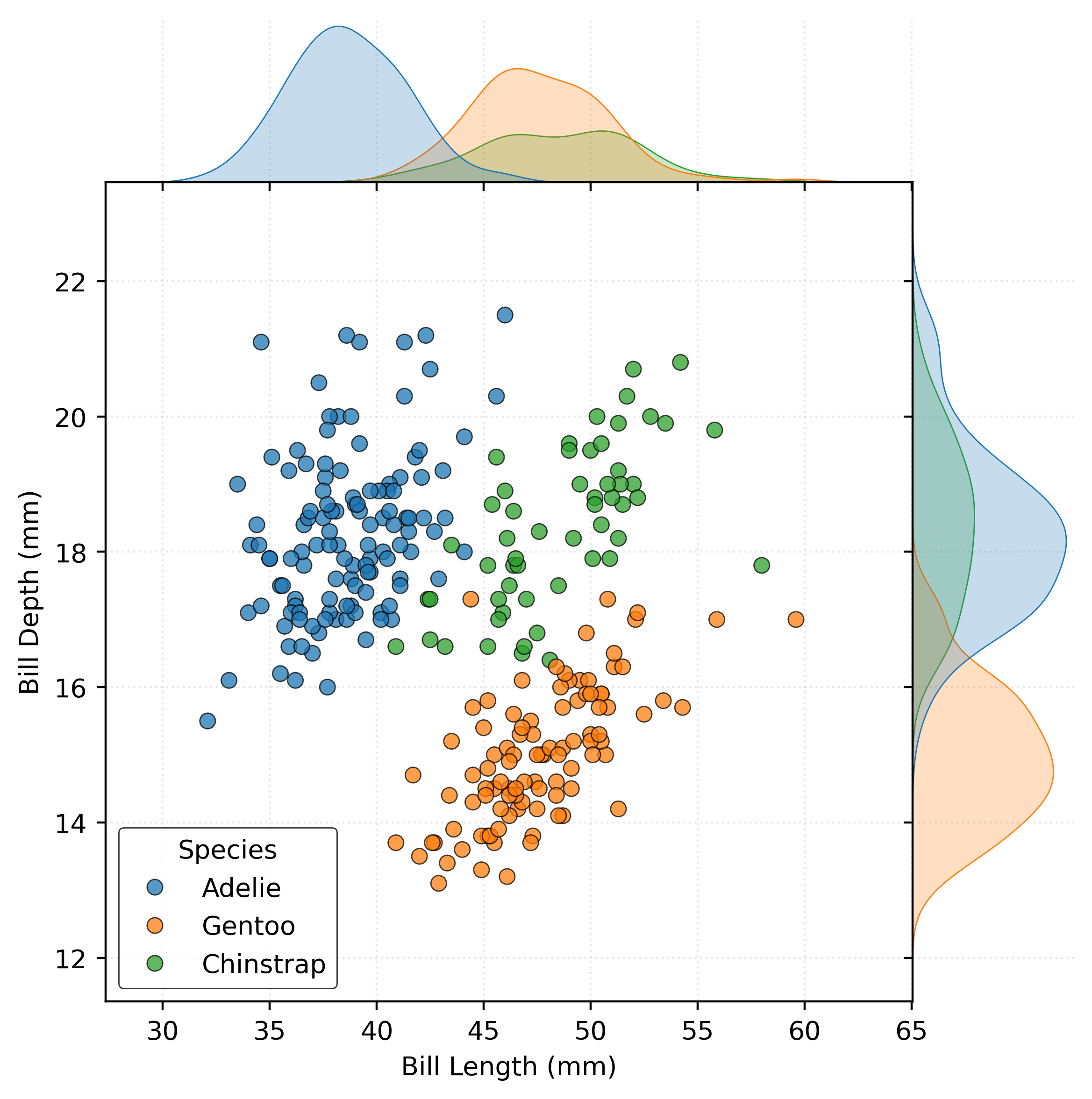
penguins_vtrain, penguins_validation = train_test_split(
penguins_train,
test_size=0.20,
random_state=42,
)numeric_features = ["bill_length_mm", "bill_depth_mm", "body_mass_g"]
categorical_features = ["sex"]
features = numeric_features + categorical_features
target = "species"X_train = penguins_train[features]
y_train = penguins_train[target]
X_test = penguins_test[features]
y_test = penguins_test[target]X_vtrain = penguins_vtrain[features]
y_vtrain = penguins_vtrain[target]
X_validation = penguins_validation[features]
y_validation = penguins_validation[target]# define preprocessing for numeric features
numeric_transformer = make_pipeline(
    SimpleImputer(strategy="median"),
    StandardScaler(),
)
# define preprocessing for categorical features
categorical_transformer = make_pipeline(
    SimpleImputer(strategy="most_frequent"),
    OneHotEncoder(),
)
# create general preprocessor
preprocessor = make_column_transformer(
    (numeric_transformer, numeric_features),
    (categorical_transformer, categorical_features),
    remainder="drop",
)validation_accuracy = []
param_grid = [1, 5, 10, 15, 20, 25, 50, 100]for k in param_grid:
mod = make_pipeline(
preprocessor,
KNeighborsClassifier(n_neighbors=k),
)
mod.fit(X_vtrain, y_vtrain)
y_pred = mod.predict(X_validation)
validation_accuracy.append(accuracy_score(y_validation, y_pred))# arrange and print validation results
validation_results = pd.DataFrame(
{
"k": param_grid,
"Accuracy": validation_accuracy,
}
)
print(validation_results)
print(f"") k Accuracy
0 1 0.98
1 5 0.98
2 10 0.98
3 15 0.96
4 20 0.96
5 25 0.96
6 50 0.93
7 100 0.84
# get best k from validation process
k_best = np.flip(param_grid)[np.argmax(np.flip(validation_accuracy))]
# create and fit the model with the best k on the (full) training data
final_model = make_pipeline(
preprocessor,
KNeighborsClassifier(n_neighbors=k_best),
)
final_model.fit(X_train, y_train)Pipeline(steps=[('columntransformer',
ColumnTransformer(transformers=[('pipeline-1',
Pipeline(steps=[('simpleimputer',
SimpleImputer(strategy='median')),
('standardscaler',
StandardScaler())]),
['bill_length_mm',
'bill_depth_mm',
'body_mass_g']),
('pipeline-2',
Pipeline(steps=[('simpleimputer',
SimpleImputer(strategy='most_frequent')),
('onehotencoder',
OneHotEncoder())]),
['sex'])])),
('kneighborsclassifier',
KNeighborsClassifier(n_neighbors=np.int64(10)))])In a Jupyter environment, please rerun this cell to show the HTML representation or trust the notebook. On GitHub, the HTML representation is unable to render, please try loading this page with nbviewer.org.
Parameters
| steps | [('columntransformer', ...), ('kneighborsclassifier', ...)] | |
| transform_input | None | |
| memory | None | |
| verbose | False |
Parameters
| transformers | [('pipeline-1', ...), ('pipeline-2', ...)] | |
| remainder | 'drop' | |
| sparse_threshold | 0.3 | |
| n_jobs | None | |
| transformer_weights | None | |
| verbose | False | |
| verbose_feature_names_out | True | |
| force_int_remainder_cols | 'deprecated' |
['bill_length_mm', 'bill_depth_mm', 'body_mass_g']
Parameters
| missing_values | nan | |
| strategy | 'median' | |
| fill_value | None | |
| copy | True | |
| add_indicator | False | |
| keep_empty_features | False |
Parameters
| copy | True | |
| with_mean | True | |
| with_std | True |
['sex']
Parameters
| missing_values | nan | |
| strategy | 'most_frequent' | |
| fill_value | None | |
| copy | True | |
| add_indicator | False | |
| keep_empty_features | False |
Parameters
| categories | 'auto' | |
| drop | None | |
| sparse_output | True | |
| dtype | <class 'numpy.float64'> | |
| handle_unknown | 'error' | |
| min_frequency | None | |
| max_categories | None | |
| feature_name_combiner | 'concat' |
Parameters
| n_neighbors | np.int64(10) | |
| weights | 'uniform' | |
| algorithm | 'auto' | |
| leaf_size | 30 | |
| p | 2 | |
| metric | 'minkowski' | |
| metric_params | None | |
| n_jobs | None |
# predict on the test data
y_test_pred = final_model.predict(X_test)

# calculate and print the test accuracy
test_accuracy = accuracy_score(y_test, y_test_pred)
print(f"Test Accuracy: {test_accuracy}")
Test Accuracy: 0.9855072463768116Footnotes
Considering missing data to be a category might seem odd, but is actually quite reasonable. We’ll give this choice more consideration in a future note when consider application to real data.↩︎