Data Splitting

Splitting, Evaluation, and Tuning

Table of Contents

• Objectives
• Python Setup
• Generalization
• Data Splitting
  • Train-Test Split
  • Train-Validation-Test Split
  • Train-Validation-Test Split Flowchart
• Test and Validation Metrics
• Example: Simulated Data
  • Data Setup
  • Create Models with KNeighborsRegressor
  • Fit Models with .fit()
  • Make Predictions with .predict()
  • Calculate Validation Metrics for Tuning
  • Refit and Calculate Test Metrics
  • Visualizing Test Results
• A Process for Supervised Learning
• Example: Automobile Fuel Efficiency
  • Data Loading and Preprocessing
  • Data Splitting
  • Model Tuning
  • Visualizing the Tuning Results
  • Model Selection and Final Evaluation
  • Discussion and Limitations

Objectives

In this note, we will discuss:

• data splitting,
• using training data for model fitting,
• using validation data for model tuning,
• and using test data for final model evaluation.

Along the way, we will outline a general procedure that will be used for almost all supervised learning tasks. We will end with an example using real data.

Python Setup

# basics
import numpy as np
import pandas as pd
import seaborn as sns
import matplotlib.pyplot as plt

# machine learning
from sklearn.model_selection import train_test_split
from sklearn.neighbors import KNeighborsRegressor
from sklearn.dummy import DummyRegressor
from sklearn.metrics import root_mean_squared_error

# data
from ucimlrepo import fetch_ucirepo

Generalization

A model generalizes well if it is able to make good predictions on unseen data.¹ Predicting on already observed data is easy!

The question is: How do we know if our models are generalizing well?

In the previous note (Regression Introduction: Comparing Models), we demonstrated the issues with using the same data to both fit a model and evaluate a model. However, our solve involved magically generating more data, a strategy that will not work in practice.

The question that we really need to ask is: How do we know if our models are generalizing well, using only data that is available?

To answer this question, we’ll again simulate some data using the simulate_sin_data function that we wrote previously.

def simulate_sin_data(n, sd, seed):
    np.random.seed(seed)
    X = np.random.uniform(low=-2 * np.pi, high=2 * np.pi, size=(n, 1))
    signal = np.sin(X).ravel()
    noise = np.random.normal(loc=0, scale=sd, size=n)
    y = signal + noise
    return X, y

However, this time we will only simulate data once, and we will not create any new data after fitting models.

X, y = simulate_sin_data(
    n=500,
    sd=0.25,
    seed=42,
)

Now the very specific question we want to answer is: How can we use only X and y to both fit a model, and evaluate its performance (how well it generalizes)?

Data Splitting

Because we cannot simply simulate new data in practice, we will instead “split” the available data into subsets, and use the different subsets for different concerns such as model fitting and model evaluation. These splits are part of standard practice in machine learning, and thus have been given specific names.

Train-Test Split

The train-test split uses the available data and randomly “splits” the (rows of the) data into two subsets:

• the train data,
• and the test data.

The train data will be used to fit (and tune) models, while the test data is used for final model evaluation.

However, we will actually need to go one level deeper.

Train-Validation-Test Split

The test data will be used for final model evaluation. Specifically, in the process we are now outlining, the test data is effectively set to the side, and only returned to after a model has been developed.

Thinking about KNN, we will need to find a good value of \(k\) to use. We will not use the test data to do this! After we find a good value of \(k\), and only then, we will use the test data to calculate metrics like RMSE to provide a final evaluation of the model.

So how do we pick \(k\)?

We will take the current (full) train data, and perform another split. We will call the resulting data the (validation) train and validation data.

Wait, there are two datasets named train? Unfortunately, yes. It’s an oddity of naming that is unfortunately common, inconsistent, and needlessly confusing, but is widely used in ML. We will disambiguate by using the parenthetical labels (full) and (validation) to signal which train set we are discussing. Over time, it will largely be clear from context, but at first, we want to avoid any potential confusion.

What will we do with each of these datasets?

• Train: The data used to train (tune and fit) models.
  • (Validation) Train: The data used to fit models during training.
  • Validation: The data used to evaluate models during training, for tuning purposes.
• Test: The data used only for a final evaluation of an already chosen model.

The term train in itself is a bit overloaded. What does it mean to train a model? Good question, but there isn’t a clear answer. You’d think you’d use the train data to train a model, and you’d be right, but remember, we have two train sets. We’ll refer to training as the action that is performed with the (full) train set, but as you will see, we will also sometimes specifically say we fit to that data.

The validation and test sets have slightly different use cases, but they are both a form of a holdout set. A holdout set is simply a dataset that is “held out” from model fitting.

Train-Validation-Test Split Flowchart

We summarize the splitting procedures in Figure 1.

flowchart TB
  A("Full Data")
  A -->|"80%"| B("(Full) Train Data")
  B -->|"80%"| D("(Validation) <br> Train Data")
  B -->|"20%"| E("Validation Data")
  A -->|"20%"| C("Test Data")

Figure 1: Flowchart that describes the train-test split and the further splitting of the train data.

An approximately 80-20 split is common for both splits, but not required. The choice of how much data to put into each set is called data budgeting. We’ll return to these details later, but the size of the split is governed by a tradeoff.

Thinking about the initial train-test split:

• With more data in the train set, models can learn patterns more effectively.
• With more data in the test set, we can better estimate a model’s future performance.

In practice, we need “enough” in both, but we’ll leave that as a topic to return to in the future. For now, an 80-20 split will be reasonable.

Test and Validation Metrics

Now that we have a desire to fit a model to some data, but calculate metrics based on holdout data, we need to update our metric definitions.

Recall our current definition of RMSE:

\[ \text{RMSE}(y, \hat{y}) = \sqrt{\frac{1}{n} \sum_{i=1}^{n} (y_i - \hat{y}_i)^2} \]

Let’s consider an updated version of this definition:

\[ \text{RMSE}(f, \mathcal{D}) = \sqrt{ \frac{1}{n_\mathcal{D}} \sum_{i \in \mathcal{D}} \left( y_i - f(x_i) \right) ^ 2} \]

Here:

• \(f\) is a function that outputs predictions. In sklearn, a function like some_model.predict().
• \(\mathcal{D}\) is a dataset, usually either the validation or test data.
• \(n_\mathcal{D}\) is the number of observations in the dataset \(\mathcal{D}\).
• \(i\) is the index of an observation (row) of the dataset \(\mathcal{D}\). \(x_i\) is the feature value(s) for this observation and \(y_i\) is the target value.

Importantly, we now need to consider both a dataset and function (learned from data) when calculating metrics.

Going forward, we will never simply refer to RMSE without qualification. Instead, we will consider one of:

• train RMSE,
• validation RMSE,
• or test RMSE.

We’re still comparing “true” values to “predicted” values, but we need to pay attention to where they come from.

Validation metrics use…

• predictions from models, \(f\), fit to (validation) train data.
• features \(x_i\) and target \(y_i\) from validation data.

Test metrics use…

• predictions from models, \(f\), fit to (full) train data.
• features \(x_i\) and target \(y_i\) from test data.

Validation metrics will be used to tune models. Test metrics will be used for final evaluation of a tuned model.

This formulation is useful for understanding test and validation metrics, however, it is cumbersome to write, and in some sense not used in practice. We will generally still refer to our previous definitions.

\[ \text{RMSE}(y, \hat{y}) = \sqrt{\frac{1}{n} \sum_{i=1}^{n} (y_i - \hat{y}_i)^2} \]

In this formulation, we will need to consider which dataset \(y\) comes from, and how \(\hat{y}\) is created.

For validation metrics:

• \(y\) is the response in the validation data.
• \(\hat{y}\) are predictions from a model fit to the (validation) train data for features \(x\) from the validation data.

For test metrics:

• \(y\) is the response in the test data.
• \(\hat{y}\) are predictions from a model fit to the (full) train data for features \(x\) from the test data.

Example: Simulated Data

To illustrate these new ideas, it will be easier to see them in action.

Data Setup

Let’s return to the data we simulated above.

X.shape, y.shape

((500, 1), (500,))

We first split the full data into a (full) train and test set using the train_test_split from sklearn.

X_train, X_test, y_train, y_test = train_test_split(
    X,
    y,
    test_size=0.20,
    random_state=42,
)

This code performs the initial train-test split using the “available” data. It takes the complete dataset (as feature array X and response array y) and randomly divides it into two subsets, each with a feature and response array.

• The resulting train set is stored as X_train and y_train.
• The resulting test set is stored as X_test and y_test.

The test_size=0.20 parameter specifies that 20% of the data should be reserved for testing, while the remaining 80% will be used for training purposes.

X_train.shape, X_test.shape

((400, 1), (100, 1))

The random_state=42 parameter ensures reproducibility. By setting this seed value, the random splitting process will produce the same train-test division every time the code is run, making results consistent across different executions.

We then repeat this process, splitting the (full) train set into a (validation) train and validation set, again using the train_test_split function.

X_vtrain, X_validation, y_vtrain, y_validation = train_test_split(
    X_train,
    y_train,
    test_size=0.20,
    random_state=42,
)

Where we previously used X and y as input, we now use X_train and y_train.

X_vtrain.shape, X_validation.shape

((320, 1), (80, 1))

With our data split, we can proceed to model tuning.

Create Models with KNeighborsRegressor

In this example, we’ll keep things simple, and as before, consider three potential values of \(k\):

• \(k = 1\)
• \(k = 10\)
• \(k = 100\)

knn_001 = KNeighborsRegressor(n_neighbors=1)
knn_010 = KNeighborsRegressor(n_neighbors=10)
knn_100 = KNeighborsRegressor(n_neighbors=100)

We initialize each of these models using KNeighborsRegressor.

Our goal is to tune a KNN model, which means we would like to determine good values of the tuning parameters like \(k\). When tuning, we determine a set of candidate models to consider, specified via potential values of tuning parameters. Here, we are considering a limited number of candidate models, but in the future, we’ll consider both more tuning parameters, and more values of them.

Fit Models with .fit()

Now, similar to the previous note, we fit each of these models to data, but different data. This time, we fit each of the models to the (validation) train data, X_vtrain and y_vtrain.

_ = knn_001.fit(X_vtrain, y_vtrain)
_ = knn_010.fit(X_vtrain, y_vtrain)
_ = knn_100.fit(X_vtrain, y_vtrain)

Make Predictions with .predict()

Like before, we can use the .predict method to make predictions.

print(knn_010.predict(X_validation))

[-0.72    0.0718 -0.7686  1.0194 -0.7585  0.957  -0.7495  0.8941  0.7542
  0.0718  0.9662  0.3956  0.9154 -0.8119  0.835   0.2383 -0.7807 -0.5975
 -0.8037  1.0089  0.9854 -0.7812 -0.2986  0.6657 -0.7855 -0.7686  0.5979
  0.9467  0.1706  0.4683 -0.8143 -0.0535 -0.8776  0.8266 -0.72    0.0185
  0.8388 -0.8998  0.0746 -0.0836  0.1706  0.8759  0.7893 -1.0632 -0.7253
  0.7876 -0.7718 -1.0151  0.5466 -0.3634 -1.0151 -0.2986  0.4454  0.971
 -1.0194  0.0369  0.9854 -0.5975  0.847   0.2239 -0.407  -0.6493  0.2946
 -0.4577  0.7624 -0.72    0.5466  1.0079  0.5922 -0.8119 -0.7177 -0.3039
  0.8738  0.7542  0.6022 -0.3634 -0.9926 -1.0151 -0.4577  0.9046]

For tuning purposes, the predictions of interests are on the validation data.

y_pred_val_001 = knn_001.predict(X_validation)
y_pred_val_010 = knn_010.predict(X_validation)
y_pred_val_100 = knn_100.predict(X_validation)

Calculate Validation Metrics for Tuning

With models fit to the (validation) train data, and predictions made for the validation data, we can now calculate the relevant metrics for tuning.

rmse_val_001 = root_mean_squared_error(y_validation, y_pred_val_001)
rmse_val_010 = root_mean_squared_error(y_validation, y_pred_val_010)
rmse_val_100 = root_mean_squared_error(y_validation, y_pred_val_100)

In this case, for each model, we calculate the validation RMSE.

print(f"Validation RMSE with k = 1:   {rmse_val_001:.3f}")
print(f"Validation RMSE with k = 10:  {rmse_val_010:.3f}")
print(f"Validation RMSE with k = 100: {rmse_val_100:.3f}")

Validation RMSE with k = 1:   0.353
Validation RMSE with k = 10:  0.261
Validation RMSE with k = 100: 0.449

Based on these results, we would select the model with the \(k = 10\).

Refit and Calculate Test Metrics

The additional split to create a validation set had the negative effect of reducing the size of the data used to fit the model. Because we are done tuning, and no longer need to withhold the validation set for model fitting, we re-fit our chosen model (with \(k=10\)) to the (full) train set to potentially improve its performance. We call this the tuned model which we will move forward with.

_ = knn_010.fit(X_train, y_train)

Now, finally, we make predictions on the test data, and calculate test RMSE.

rmse_test_010 = root_mean_squared_error(y_test, knn_010.predict(X_test))
print("Test RMSE with k = 10:", rmse_test_010)

Test RMSE with k = 10: 0.2720220479053038

The test RMSE is a final quantification of our tuned model’s performance. Importantly, we did not use the test data until the very end, after we already developed our model.

A bit later, we will discuss data leakage. At the moment, it may seems trivially easy to keep the test data separated from the model tuning process. However, as we move towards more realistic examples, we will identify subtle ways you might accidentally “peek” at the test data and spoil your model tuning process.

Visualizing Test Results

For good measure, we’ll take a look at a residuals versus predicted plot, using the test data.

test_residuals = y_test - knn_010.predict(X_test)

# setup figure
fig, ax = plt.subplots()

# x values to make predictions at for plotting purposes
x_plot = np.linspace(-2 * np.pi, 2 * np.pi, 1000).reshape((-1, 1))

# create scatterplot for KNN model
ax.scatter(knn_010.predict(X_test), test_residuals, alpha=0.50, c="tab:gray")
ax.axhline(0)
ax.set_xlabel("Predicted")
ax.set_ylabel("Residuals")
ax.set_aspect("equal")

# show figure
plt.show()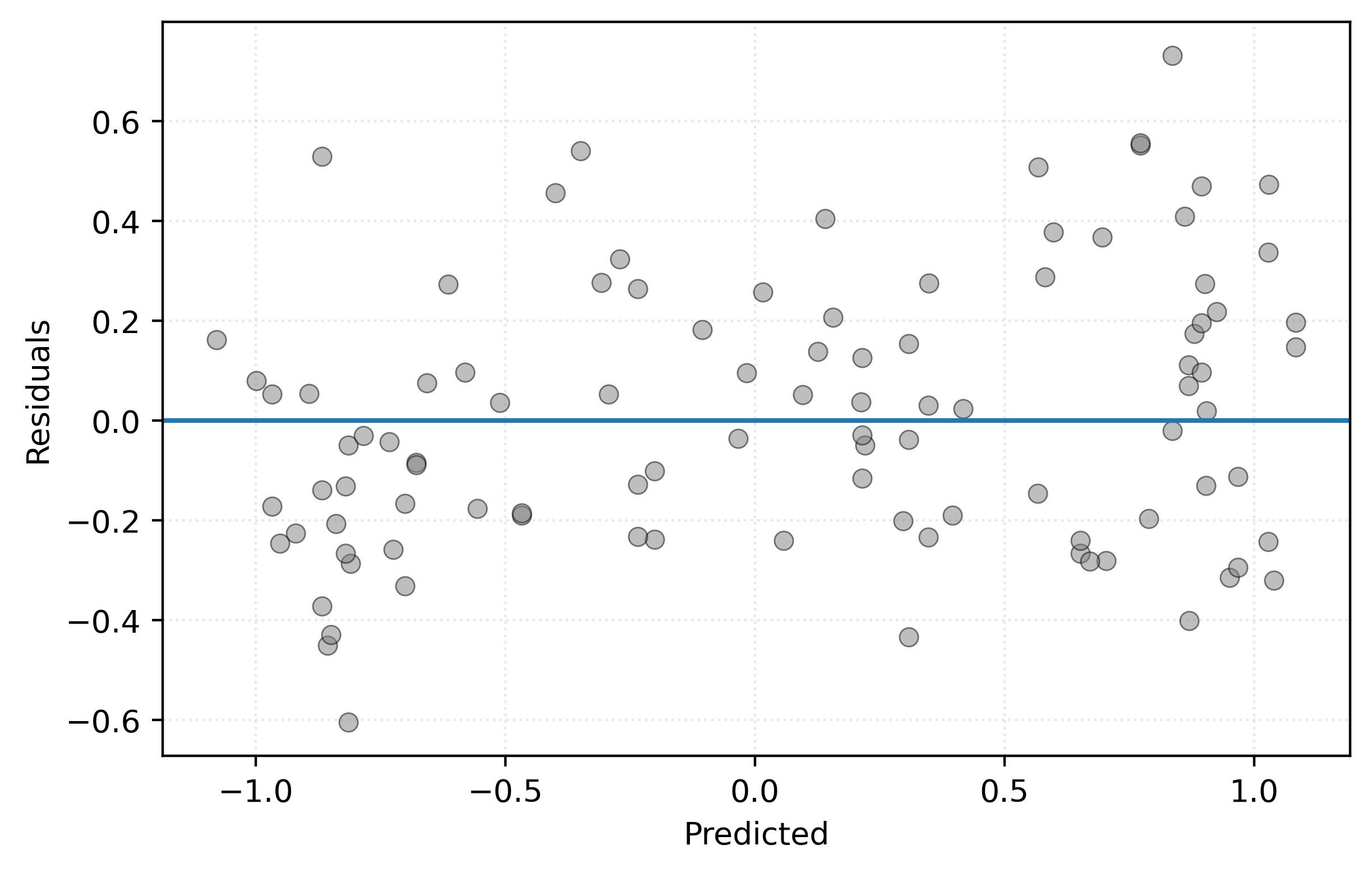

Figure 2: Residuals versus predicted values plot for the KNN regression model with \(k=10\). The residuals appear randomly scattered around zero with no clear patterns, indicating the model is not exhibiting systematic bias at different prediction levels.

Like before, we don’t see any meaningful pattern, so this seems to be at least a reasonably valid model.

A Process for Supervised Learning

Figure 3 summarizes a process that we will use for most supervised learning tasks going forward.

flowchart TB
    Pipeline{ML Pipeline} --> Model{Tuned Model}
    Model -- Predictions --> Metric[Final Evaluation]
    Estimator["Estimator"] --> Pipeline
    Data[(Data)] --> TrainData[(Train Data)]
    Data --> TestData[(Test Data)]
    TrainData -- Train Features --> Pipeline
    TrainData -- Train Target --> Pipeline
    TestData -- Test Features --> Model
    TestData -- Test Target --> Metric

Figure 3: Flowchart describing the supervised learning process.

In the previous simulation example, we applied this process as follows:

1. Train-test split the available data.
2. Further split the (full) train data into (validation) train and validation datasets.
3. Fit all candidate models (in this case, three KNN models) to the (validation) train dataset.
4. Calculate validation RMSE for each model.
5. Choose the model with the lowest validation RMSE. Call this the tuned model.
6. Fit the tuned model to the (full) train dataset.
7. Calculate test RMSE for the tuned model.

In the flowchart, steps 2 through 6 all happen in the “ML Pipeline” item. As we move forward in the course, we will essentially be looking at that particular step in detail. We will both add steps (cross-validation) and make the process conceptually more complicated, but also see how sklearn can make it easy to express in code.

Remember, in general:

• Validation metrics are for tuning and selecting models, often via their tuning parameters.
• Test metrics are for reporting the performance of a selected model.

Example: Automobile Fuel Efficiency

Now we’ll apply the this supervised learning process to a real-world dataset: the Auto MPG dataset, which contains information about automobile fuel efficiency and various car characteristics.

To follow along, we provide a notebook with starter code:

• Tuning KNN for Regression with the UCI Auto MPG Data

Our goal is to create a model that can predict fuel efficiency from vehicle characteristics.

Data Loading and Preprocessing

auto_mpg = fetch_ucirepo("Auto MPG")

We load the Auto MPG dataset using the fetch_ucirepo function, which provides access to datasets from the UCI Machine Learning Repository.

X = auto_mpg.data.features
y = auto_mpg.data.targets["mpg"]

We extract the features (car characteristics like engine size, weight, etc.) into X and the target variable (fuel efficiency in miles per gallon) into y.

What is this data exactly? Any good dataset should also include a data dictionary, which describes the data, in particular noting background information such as how it was collected, and most importantly, descriptions of the available variables. Unfortunately, the provided variable descriptions are lacking, so we create our own.

Each row of the dataset describes characteristics for a make and model of automobile (“Toyota Camry”) for a particular model year.

• mpg
  • fuel efficiency for city driving in miles per gallon
• displacement
  • engine displacement (size) in cubic inches
• cylinders
  • number of engine cylinders
• horsepower
  • engine horsepower rating
• weight
  • vehicle weight in pounds
• acceleration
  • time to accelerate from 0 to 60 mph in seconds
• model_year
  • model year of the vehicle (70 - 82, representing 1970 - 1982)
• origin
  • origin of manufacture (1 for US, 2 for Europe, 3 for Japan)

A few of the horsepower values are missing, so for this analysis, we will simply remove them.

not_missing = ~X["horsepower"].isna()

X = X[not_missing].copy()
y = y[not_missing].copy()

We handle missing data by identifying rows where the “horsepower” feature is not missing and filtering our dataset to include only complete observations. This ensures our models won’t encounter missing values during training.

That last bit of preprocessing that we performed, removing the missing values, broke the most important rule: do not use test data before you’ve chosen a model. But wait, you’re probably thinking: We don’t have test data yet! Correct, but some of the data we just removed could have been test data eventually. This is an example of subtle data leakage.

For now, we need to perform this simplification for illustrative purposes. But soon, we’ll talk about preprocessing in detail, and explain how to properly deal with missing data.

A general heuristic you should keep in mind: split off the test data as soon as possible, and any preprocessing decisions should be made based only on the train data.

Data Splitting

Following our established process, we perform the train-test split:

X_train, X_test, y_train, y_test = train_test_split(
    X,
    y,
    test_size=0.2,
    random_state=42,
)

This creates our initial 80-20 split between (full) train and test data. Now that we’ve split off the test data, we should perform some exploratory data analysis on the train data.²

print(y_train[:5])

260   18.60
184   25.00
174   18.00
64    15.00
344   39.00
Name: mpg, dtype: float64

X_train.dtypes

displacement    float64
cylinders         int64
horsepower      float64
weight            int64
acceleration    float64
model_year        int64
origin            int64
dtype: object

Let’s briefly explore the relationships between the features and the response to better understand this data:

# prepare data for seaborn
train_data = X_train.copy()
train_data["mpg"] = y_train
# convert origin to categorical with proper labels
origin_labels = {1: "US", 2: "Europe", 3: "Japan"}
train_data["origin"] = train_data["origin"].map(origin_labels).astype("category")

# get features to plot (excluding origin since we use it for coloring)
features_to_plot = [col for col in X_train.columns if col != "origin"]

# create 2x3 subplot grid
fig, axes = plt.subplots(2, 3, figsize=(15, 8))

# create nice labels with units
feature_labels = {
    "displacement": "Displacement (cubic inches)",
    "cylinders": "Cylinders",
    "horsepower": "Horsepower",
    "weight": "Weight (pounds)",
    "acceleration": "Acceleration (0-60 mph, seconds)",
    "model_year": "Model Year",
}

# create scatter plot for each feature, colored by origin
for i, feature in enumerate(features_to_plot):
    row = i // 3
    col = i % 3
    sns.scatterplot(
        data=train_data,
        x=feature,
        y="mpg",
        hue="origin",
        edgecolor="k",
        alpha=0.7,
        ax=axes[row, col],
    )
    axes[row, col].set_xlabel(feature_labels[feature])

    # only add y-label for first column of each row
    if col == 0:
        axes[row, col].set_ylabel("Fuel Efficiency (mpg)")
    else:
        axes[row, col].set_ylabel("")

    # update legend title to title case
    legend = axes[row, col].get_legend()
    if legend:
        legend.set_title("Origin")

plt.show()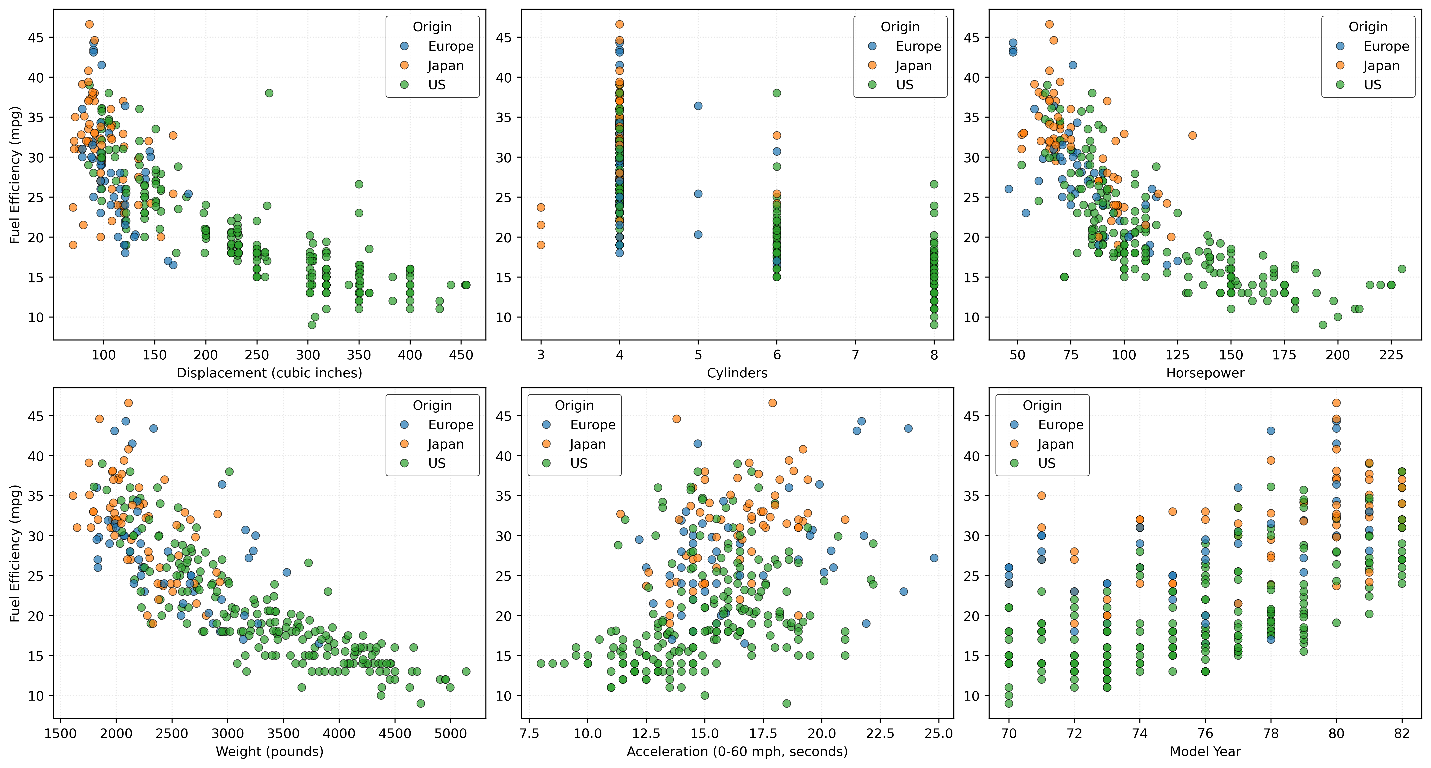

Figure 4: Scatterplots showing the relationship between features and fuel efficiency (mpg), colored by origin of manufacture.

Figure 4 shows some clear relationships: larger engines, more cylinders, higher weight, and more horsepower all correlate with lower fuel efficiency. Japanese cars tend to be more fuel-efficient, while US cars, which are generally heavier and more powerful, tend to be less fuel-efficient. Newer model years show improved efficiency over time.

We then further split the train data to create validation data for tuning:

X_vtrain, X_validation, y_vtrain, y_validation= train_test_split(
    X_train,
    y_train,
    test_size=0.2,
    random_state=42,
)

Model Tuning

Rather than considering just three values of \(k\) as in our simulation example, we’ll systematically evaluate a wide range of \(k\) values to find a good choice:

k_values = range(1, 202, 5)
validation_rmse_scores = []

We define a range of \(k\) values from 1 to 201 (stepping by 5) and create an empty list that will store the corresponding validation RMSE scores.

for k in k_values:
    knn = KNeighborsRegressor(n_neighbors=k)
    knn.fit(X_vtrain, y_vtrain)
    y_pred = knn.predict(X_validation)
    rmse = root_mean_squared_error(y_validation, y_pred)
    validation_rmse_scores.append(rmse)

For each candidate \(k\) value, we:

1. Create a KNN regressor with that \(k\).
2. Fit that model to the (validation) training data.
3. Make predictions on the validation data.
4. Calculate the validation RMSE.
5. Store the validation RMSE for comparison.

This loop implements the core of our tuning process, evaluating each candidate model.

Visualizing the Tuning Results

fig, ax = plt.subplots(figsize=(8, 5))
ax.scatter(k_values, validation_rmse_scores, c="tab:gray", s=15)
ax.plot(k_values, validation_rmse_scores, zorder=-1, lw=1)
ax.set_xlabel("$k$ (Number of Neighbors)")
ax.set_ylabel("Validation RMSE")
plt.show()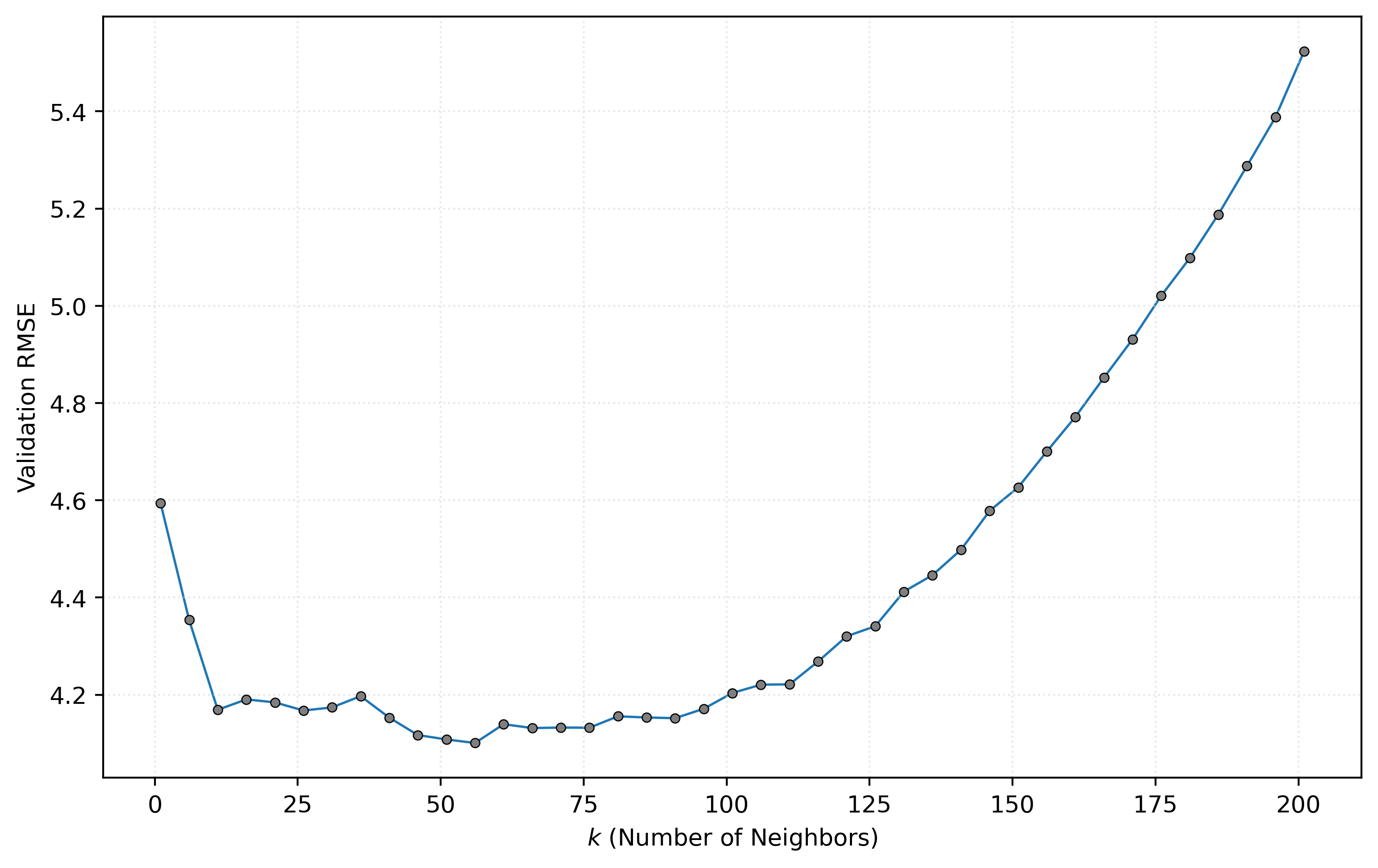

Figure 5: Validation RMSE vs \(k\) for KNN regression models fit to the Auto MPG dataset.

Figure 5 shows how validation RMSE varies with different values of \(k\). In a future note, we will discuss graphics like this in detail. For now, you should notice the shape of the curve. In particular, the U-shape has “large” validation RMSE values when \(k\) is small or large, with “small” validation RMSE values in between.

Model Selection and Final Evaluation

best_k = k_values[np.argmin(validation_rmse_scores)]
best_k

56

We identify the \(k\) value that produced the lowest validation RMSE. The np.argmin function returns the index of the minimum value, which we use to extract the corresponding \(k\) from our range. With this, we can create the final tuned model by re-fitting to the (full) train data.

knn = KNeighborsRegressor(n_neighbors=best_k)
_ = knn.fit(X_train, y_train)

Then, finally, we can evaluate this tuned model’s performance. Here, we calculate its test RMSE.

root_mean_squared_error(y_test, knn.predict(X_test))

4.207430453194762

For a more detailed bit of model introspection, we also create a residuals versus predicted plot, using the test data.

y_pred_test = knn.predict(X_test)
test_residuals = y_test - y_pred_test

# setup figure
fig, ax = plt.subplots()

# x values to make predictions at for plotting purposes
x_plot = np.linspace(np.min(y_pred_test), np.max(y_pred_test)).reshape((-1, 1))

# create scatterplot for KNN model
ax.scatter(y_pred_test, test_residuals, alpha=0.50, c="tab:gray")
ax.axhline(0)
ax.set_xlabel("Predicted")
ax.set_ylabel("Residuals")

# show figure
plt.show()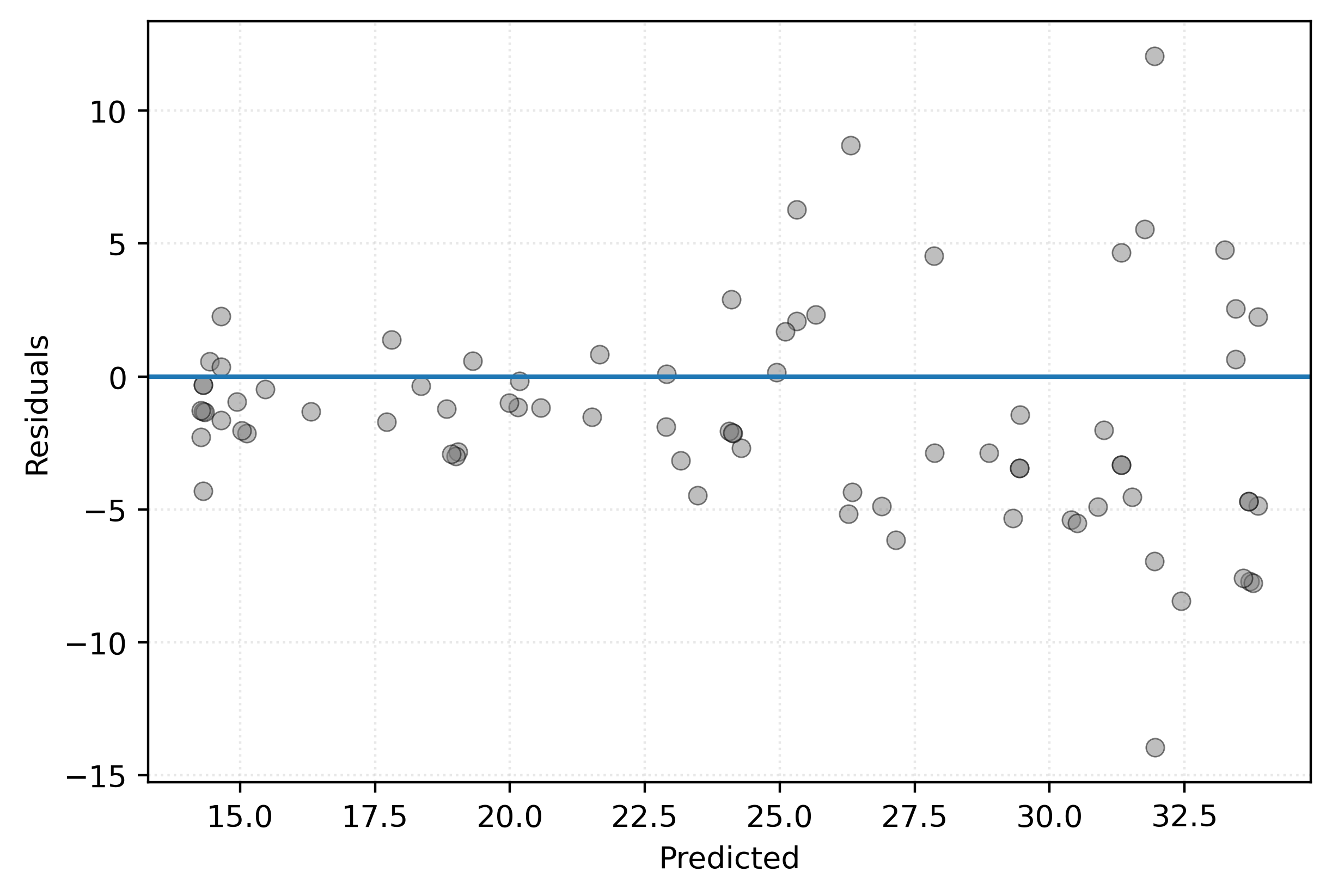

Figure 6: Residuals versus predicted plot for the tuned KNN regression model for the Auto MPG data.

Figure 6 shows points scattered about 0, however, we see an increasing spread as the predicted values increase. This indicates that we are less confident in predicting fuel efficiency for highly efficient vehicles.

Discussion and Limitations

Is this a good model? Should it be used in practice? If so, what if any limitations should be considered?

TODO

Discuss:

TODO: 4.2, is that good? (compare to R^2) TODO: RMSE vs MAPE TODO: 1993!! TODO: distance! TODO: EDA of train data?! TODO: df versus array (.to_numpy)

• methods to describe:
  • .fit
  • .predict
  • .score
  • .get_params
  • () .kneighbors
• TODO: conditional distribution? conditional mean?
• TODO: When we overfit, which is one way to generalize poorly, we have accidentally learned the noise.

Footnotes

1. We says “generalizes” because it works well in general, rather than just for the specific data available to fit a model.

2. Exploring the test data is cheating, and will leak data.