graph TD
    A[Machine Learning] --> B[Supervised Learning]
    A --> C[Unsupervised Learning]
    A --> D[Reinforcement Learning]

    B --> E[Regression]
    B --> F[Classification]

    style A color:#000
    style B color:#000
    style C color:#000
    style D color:#000
    style E fill:#e1f5fe,color:#000
    style F fill:#e1f5fe,color:#000
Machine Learning Overview
Paradigms, Tasks, and Usage
Objectives
In this note, we will discuss:
- machine learning paradigms and their distinguishing characteristics,
- the supervised learning tasks regression and classification,
- and some unsupervised learning tasks including clustering, dimension reduction, anomaly detection, and density estimation.
We will close with a discussion of when it is appropriate to put the various machine learning tasks in practice.
Machine Learning Paradigms
Machine learning can be broadly categorized into three main paradigms:
Supervised Learning uses labeled data - we have both input features, \(X\), and known target outputs, \(y\). The goal is to learn a mapping from inputs to outputs.
Unsupervised Learning works with unlabeled data - we only have input features, \(X\), without known target outputs. The goal is to discover hidden patterns or structure in the data.
Reinforcement Learning learns through interaction with an environment, receiving rewards or penalties for actions. This paradigm is beyond the scope of CS 307.
Supervised Learning
In supervised learning, we separate the available columns into input columns (features) and a single output column (target). The goal is to learn a function that maps from the input features to the target output, so we can make predictions on new, unseen data.
By convention, we use \(X\) for input, and \(y\) for output. Beyond that, there are several additional names given to the input and output.
- Input \(X\) - Features, Predictors, Independent Variables
- Output \(y\) - Target, Response, Dependent Variables
In machine learning, and in CS 307, there is a preference for using features and target.1
What distinguishes the regression and classification tasks? The (statistical) data type of the target.
Regression
The regression task seeks to predict a numeric (continuous) target variable given the available features.
Potential examples include:
- Estimating apartment rent based on neighborhood, amenities, and size
- Predicting credit scores based on financial history, income, and level of education
- Predicting college GPA based on high school grades and SAT scores
- Estimating blood pressure based on age, weight, exercise habits, and diet
- Estimating delivery times based on distance, traffic, and weather
- Predicting crop yield based on soil conditions, weather, and farming practices
What does this look like? Let’s consider some generic data with features \(x_1\), \(x_2\), and \(x_3\) and response \(y\). The features \(x_1\), \(x_2\), and \(x_3\) could represent things like age, weight, etc, and the response \(y\) could represent blood pressure. That won’t be the case here. We’re just noting that the \(x_1\), \(x_2\), and \(x_3\) variables generally represent some features, and \(y\) represents some response. Let’s look at a few samples of a larger dataset.
| \(x_1\) | \(x_2\) | \(x_3\) | \(y\) |
|---|---|---|---|
| -0.47 | -1.58 | 2.92 | -1.06 |
| 0.54 | 5.66 | 3.66 | -0.61 |
| -0.46 | 2.92 | 4.56 | 0.16 |
| -0.47 | 1.24 | 7.85 | 1.13 |
| 0.24 | -4.32 | 2.00 | 0.92 |
| -1.91 | -4.32 | 5.14 | 0.82 |
| -1.72 | -5.55 | 5.92 | 0.75 |
| -0.56 | 4.60 | 0.46 | -1.12 |
| -1.01 | 1.27 | 6.08 | 0.98 |
| 0.31 | 2.61 | 1.71 | 0.31 |
Do you see a pattern? If you saw new feature data, could you make a good prediction for \(y\)?
| \(x_1\) | \(x_2\) | \(x_3\) |
|---|---|---|
| -1.79 | -2.25 | 8.82 |
You probably have no idea if there is a pattern here. We only gave you ten samples, but with 100 more, you still probably wouldn’t see a pattern.
Let’s look at more of this data, visually instead of as a table.
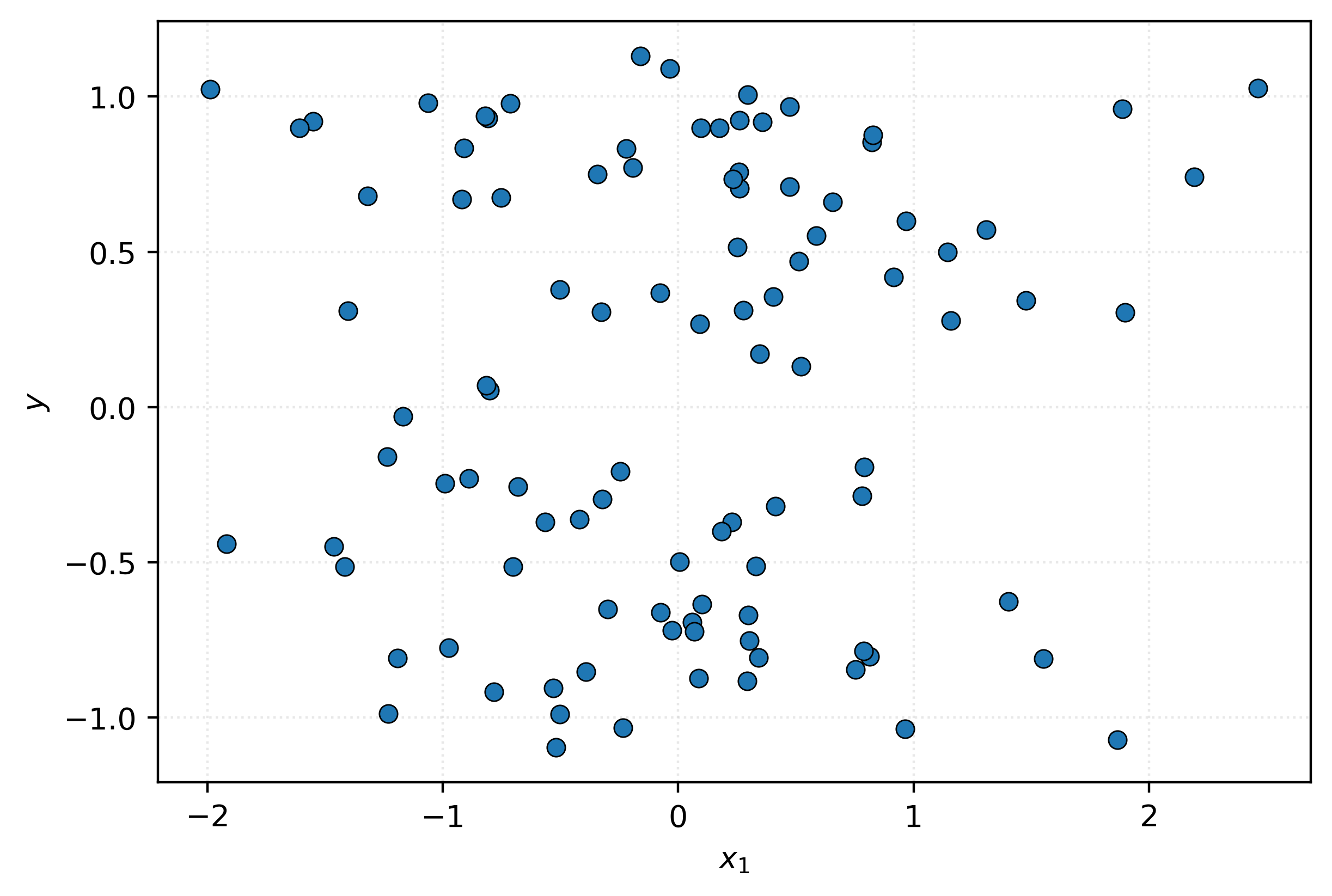
This scatterplot doesn’t seem to suggest a pattern between \(x_1\) and \(y\). It seems like nothing but noise. Let’s try a different feature.
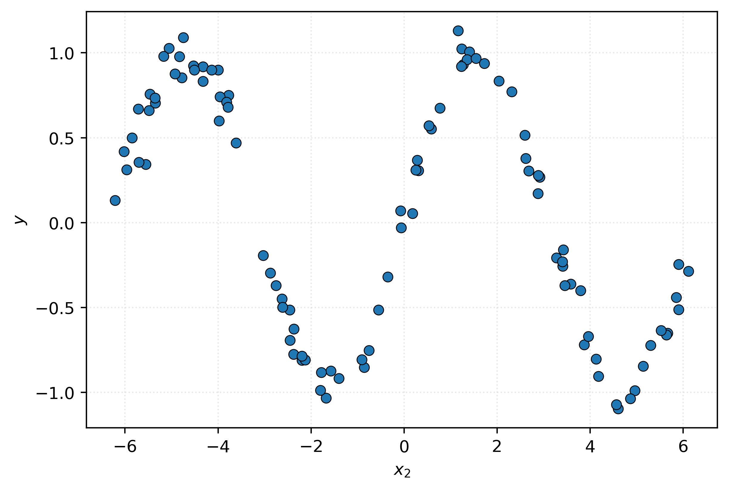
And there it is, a pattern emerges! With this, if we return to the new feature data above, with \(x_2 = -2.25\), you can probably make a pretty reasonable prediction for the value of \(y\).2
Now of course in practice, two things here are wildly unrealistic. In practice, relationships will rarely if ever be so plainly obvious. Also in practice, the whole point is for machines carry out this task! Human inspection of visualizations is useful, but imagine data with hundreds, thousands, even millions of features. We all have better things to do than look for needles in haystacks all day.
We need to learn methods for machines to uncover and learn these patterns. We’ll get there soon!
Classification
The classification task seeks to predict a categorical target variable, or more specifically, estimate the probability of each potential category, given the available features.
Potential examples include:
- Predicting whether an email is spam or not spam based on number of exclamation marks, sender domain, subject length, and presence of certain keywords
- Determining if a credit card transaction is fraudulent based on transaction amount, merchant category, time of day, and distance from previous transaction
- Classifying images as containing a cat, dog, or bird based on individual pixel intensity values
- Diagnosing whether a patient has a disease based on blood pressure, cholesterol level, age, and family history
For each, classification will often go one step further, and estimate the probability of each category of the response, given the features. In the spam or ham (not-spam) example, rather than simply predicting if an email is spam given its characteristics, we might want to know the probability of spam and the probability of ham.
Let’s again look at some example data.
| \(y\) | \(x_1\) | \(x_2\) |
|---|---|---|
| C | 6.85 | 6.01 |
| C | 5.85 | 6.18 |
| B | 15.11 | 15.76 |
| C | 6.15 | 5.41 |
| A | 10.73 | 20.10 |
| A | 10.02 | 22.56 |
| A | 12.07 | 22.78 |
| B | 13.33 | 13.57 |
| B | 15.37 | 11.44 |
| A | 10.03 | 21.55 |
Do you see a pattern? If you saw new feature data, could you make a good prediction for \(y\)?
| \(x_1\) | \(x_2\) |
|---|---|
| 6.69 | 10.94 |
Like before, this is pretty much a fool’s errand. Let’s investigate the data visually.
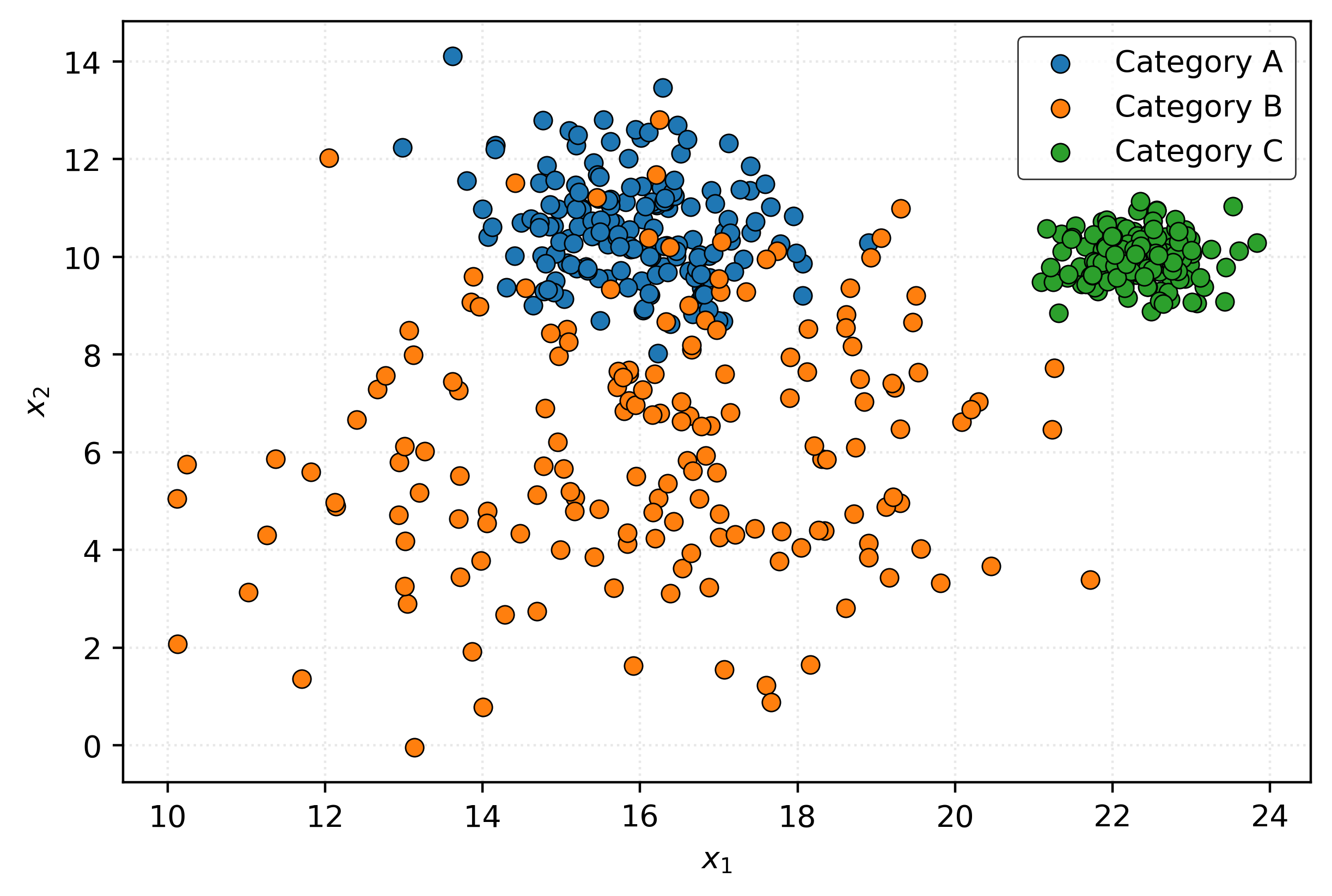
Now we can see some relationship between the features and the response. Let’s consider three new samples:
- \((x_1, x_2) = (23, 10)\)
- \((x_1, x_2) = (16, 4)\)
- \((x_1, x_2) = (16, 10)\)
For each, can you make a prediction for \(y\)?
- For \((23, 10)\), you’ll probably say \(C\) (green).
- For \((16, 4)\), you’ll probably say \(B\) (orange).
- For \((16, 10)\), you’ll probably say \(A\) (blue).
However, would you be equally confident about each of those predictions? Hopefully not!
When predicting at \((x_1, x_2) = (23, 10)\), you probably feel pretty good about your prediction of \(C\). But when predicting at \((x_1, x_2) = (16, 10)\), you’re making a decent prediction, but you wouldn’t bet the farm.3 You could imagine a new sample here having response \(B\) or \(A\) with some frequency.
Many classification methods will not only make predictions, but give you an estimation of certainty, in the the form of a probability.
For example, at \((x_1, x_2) = (23, 10)\), because you are quite confident that the response would be \(C\), you might assign probabilities like this:
- \(P(Y = A \mid (x_1, x_2) = (23, 10)) = 0.00\)
- \(P(Y = B \mid (x_1, x_2) = (23, 10)) = 0.01\)
- \(P(Y = C \mid (x_1, x_2) = (23, 10)) = 0.99\)
But at \((x_1, x_2) = (16, 10)\), because there is much more uncertainty, you might assign probabilities like this:
- \(P(Y = A \mid (x_1, x_2) = (16, 10)) = 0.75\)
- \(P(Y = B \mid (x_1, x_2) = (16, 10)) = 0.25\)
- \(P(Y = C \mid (x_1, x_2) = (16, 10)) = 0.00\)
You predict \(A\) because it is most likely, but you allow for some possibility that the response could be \(B\).
Like regression, throughout the course, we will learn classification methods that attempt to carry out a similar analysis, but automatically.
Unsupervised Learning
In unsupervised learning, we work with data that has no known target or response variable. Unlike supervised learning where we have both features \(X\) and a target \(y\) to learn from, unsupervised learning only has features \(X\). The goal is to discover hidden patterns, structures, or relationships within the data itself.
Since there is no “correct answer” to learn from, unsupervised learning tasks focus on understanding the underlying structure of the data. Unlike supervised learning where the response variable can guide correctness, it is much more difficult to evaluate the performance of unsupervised learning methods. Common unsupervised learning tasks include:
- Clustering - grouping similar samples
- Dimension Reduction - simplifying high-dimensional data (many features) by reducing the number of features but maintaining as much information as possible
- Anomaly Detection - finding unusual samples
- Density Estimation - understanding data distributions
Clustering
The clustering task seeks to group similar samples together based on their features, without knowing the true groupings (which may not exist) ahead of time. The goal is to discover natural clusters or segments within the data.
Potential examples include:
- Grouping customers based on transaction amounts, frequency, and product categories
- Segmenting website users based on page views, session durations, and click patterns
- Identifying neighborhoods based on income, education level, and housing prices
- Clustering genes based on similar expression levels across different conditions
- Defining “functional” NBA player positions based on their season-level statistics like shots taken, shots made, etc4
Let’s look at some example data and attempt to cluster it.
| \(x_1\) | \(x_2\) |
|---|---|
| 6.65 | 7.52 |
| 6.99 | 10.31 |
| 6.28 | 9.44 |
| 9.54 | 6.53 |
| 9.53 | 7.54 |
| 7.09 | 8.59 |
| 6.50 | 5.86 |
| 7.58 | 6.77 |
| 10.24 | 5.09 |
| 5.77 | 5.77 |
Do you see any natural groupings in this data? It’s probably too difficult to tell from just a table.
Let’s visualize this data:
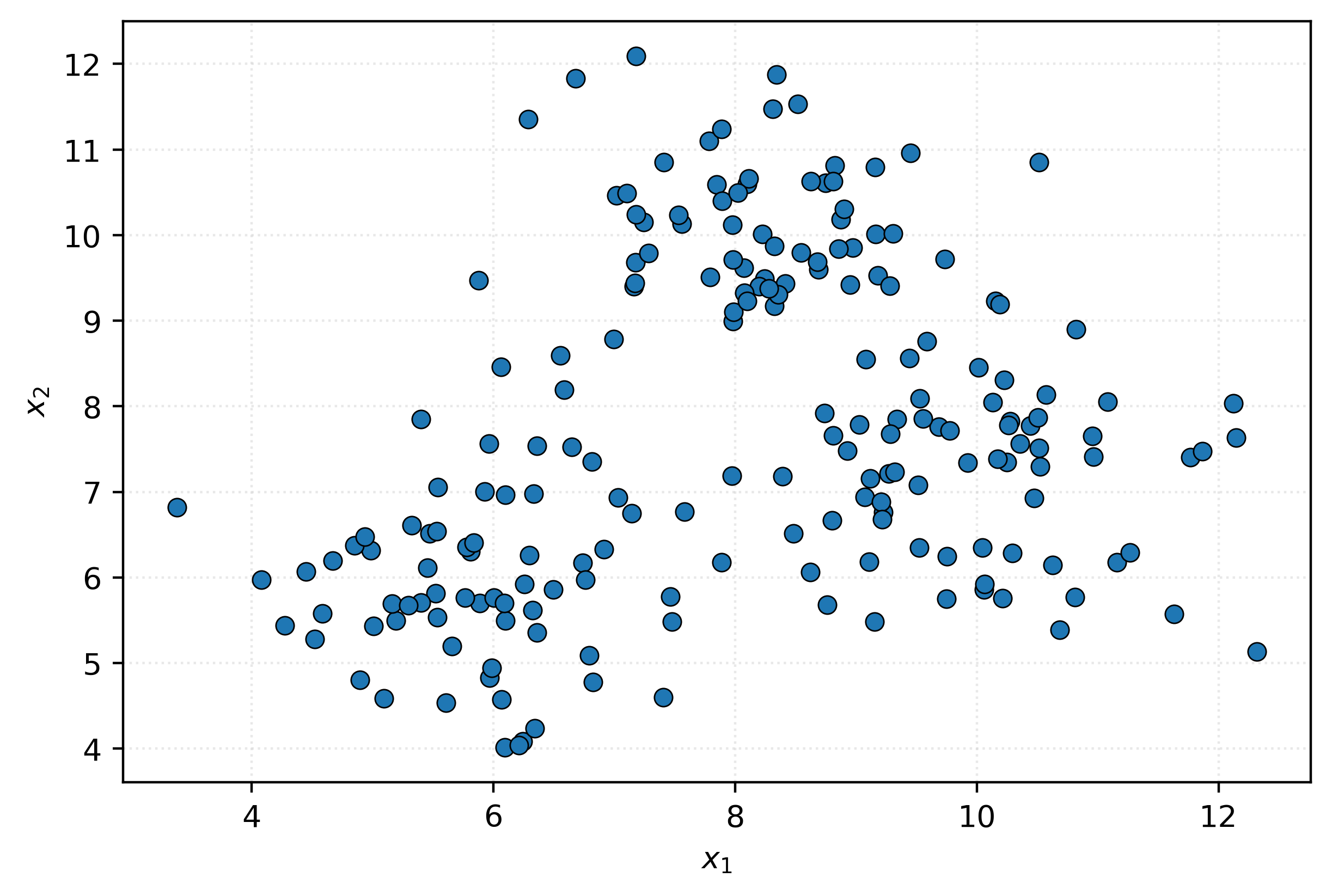
Can you see any potential groupings now? It seems there might be three data “blobs” that appear when we visualize this data. Let’s apply a clustering algorithm to see a potential categorization of this data using three groups:
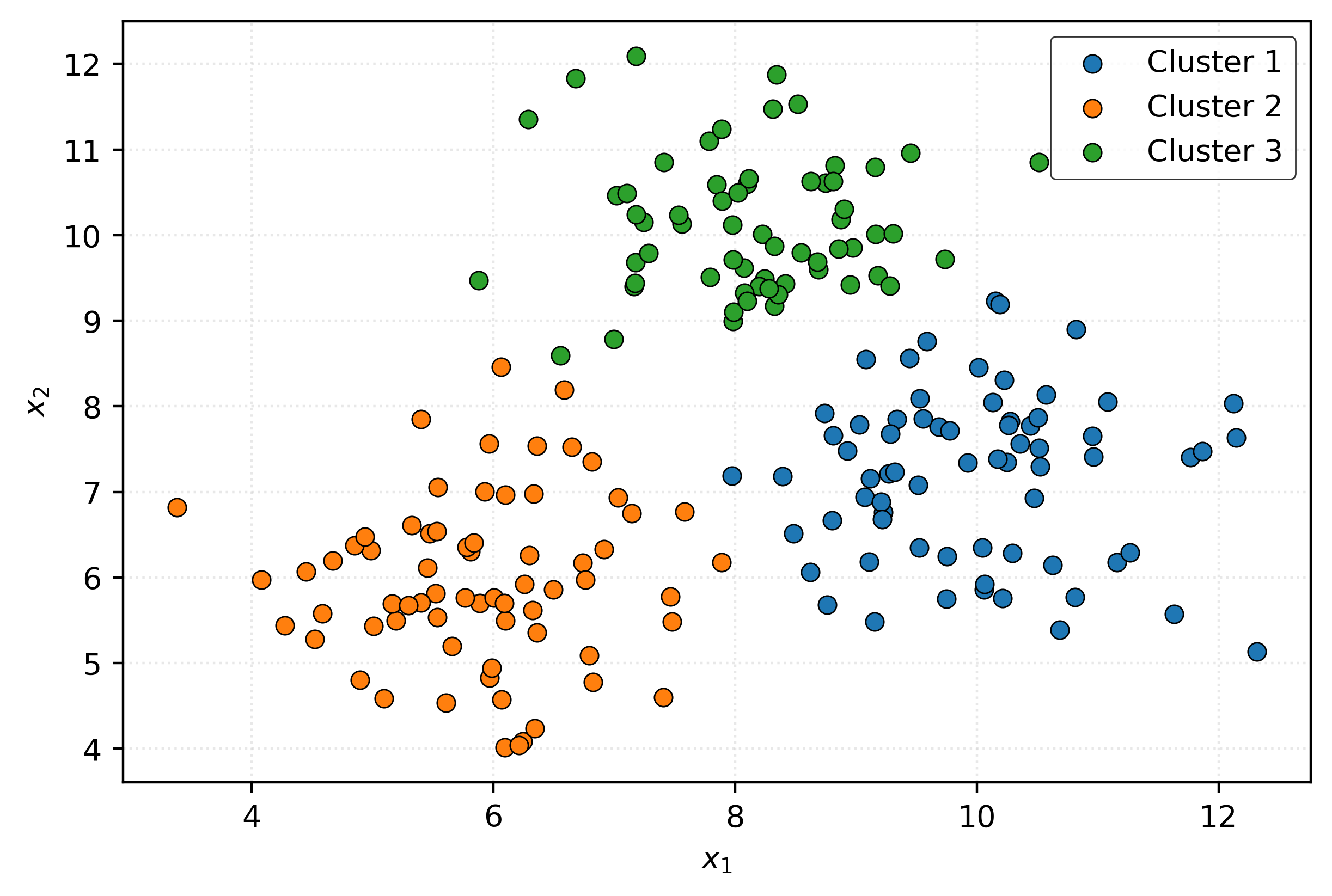
Is this clustering any good? Who knows?
Dimension Reduction
The dimension reduction task seeks to reduce the number of features in a dataset while preserving as much important information as possible. This is useful when working with high-dimensional data that may be difficult to visualize, computationally expensive to process, or contain redundant information.
[[  5.47   2.37  -7.73 ...  11.56   5.39   8.3 ]
 [  1.85   4.18   4.24 ...   6.95  -0.15  -1.62]
 [ -4.84   8.26   4.27 ...   1.91   1.85   7.16]
 ...
 [ 22.32   7.6   11.86 ...  -7.08 -14.94  -5.03]
 [  6.99 -11.2   -3.54 ...   7.54  17.32   0.19]
 [-13.91   0.62  -4.8  ...  -7.46  -8.18  -4.08]]
Suppose we have a reasonably large NumPy array, in this case 50 features for each of 500 samples.
(500, 50)We won’t bother asking if you see a way to reduce the number of columns, we know you can’t. Let’s try our usual trick of visualizing the data. We’ll create a scatterplot of the first two columns.
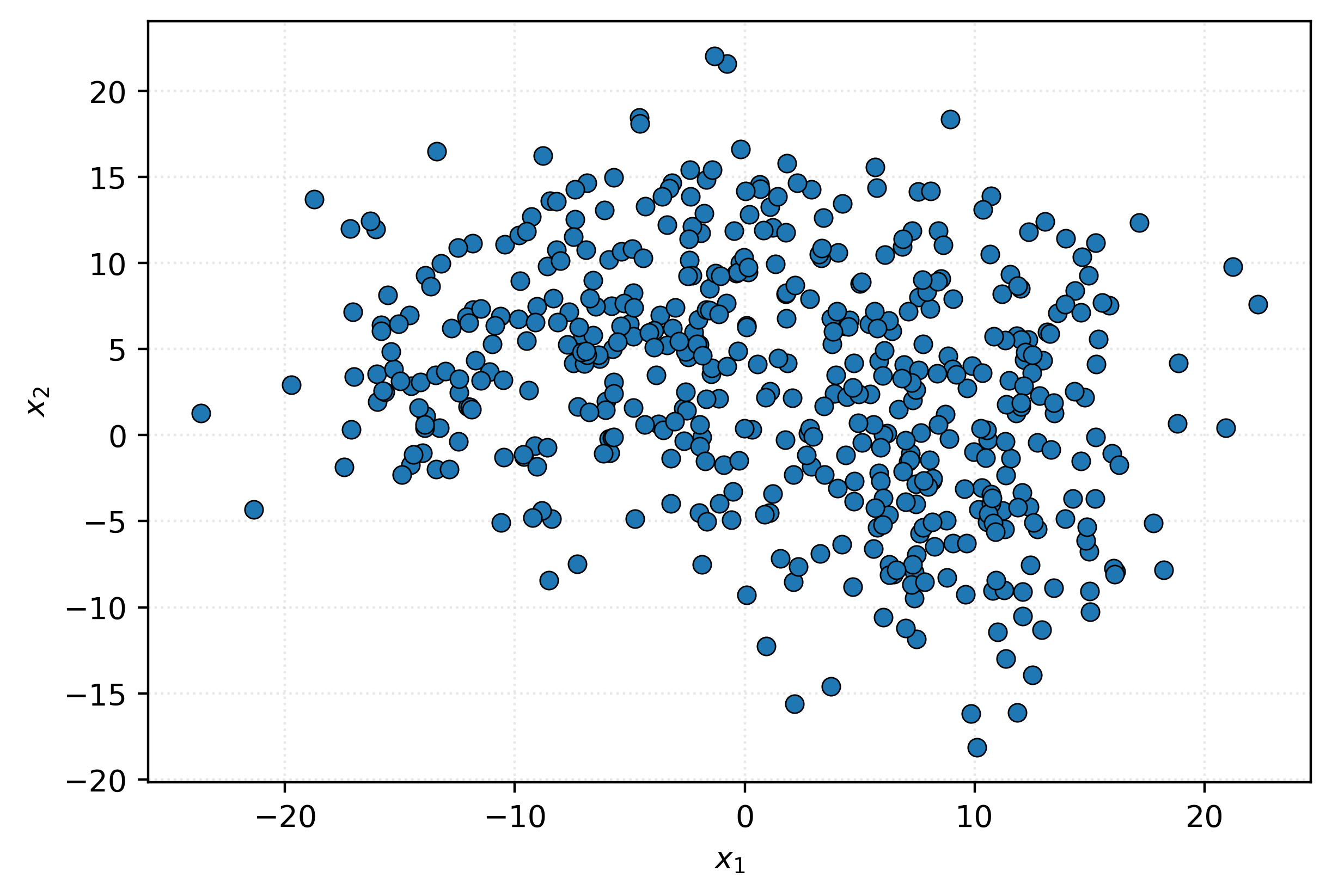
Nothing interesting there. Let’s try columns two and three.
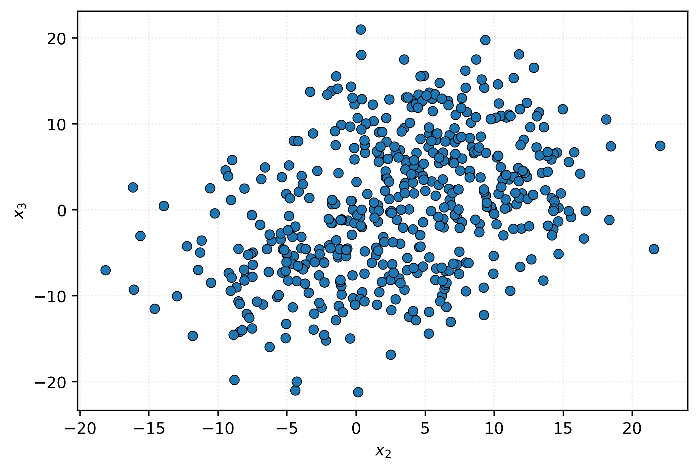
That doesn’t seem like anything either.
Now, we’ll use a dimension reduction technique to take the original 50 features, and compress them into just two features. Behind the scenes, we are using Principal Component Analysis (PCA), and thus these new features are called principal components. We plot these two components.
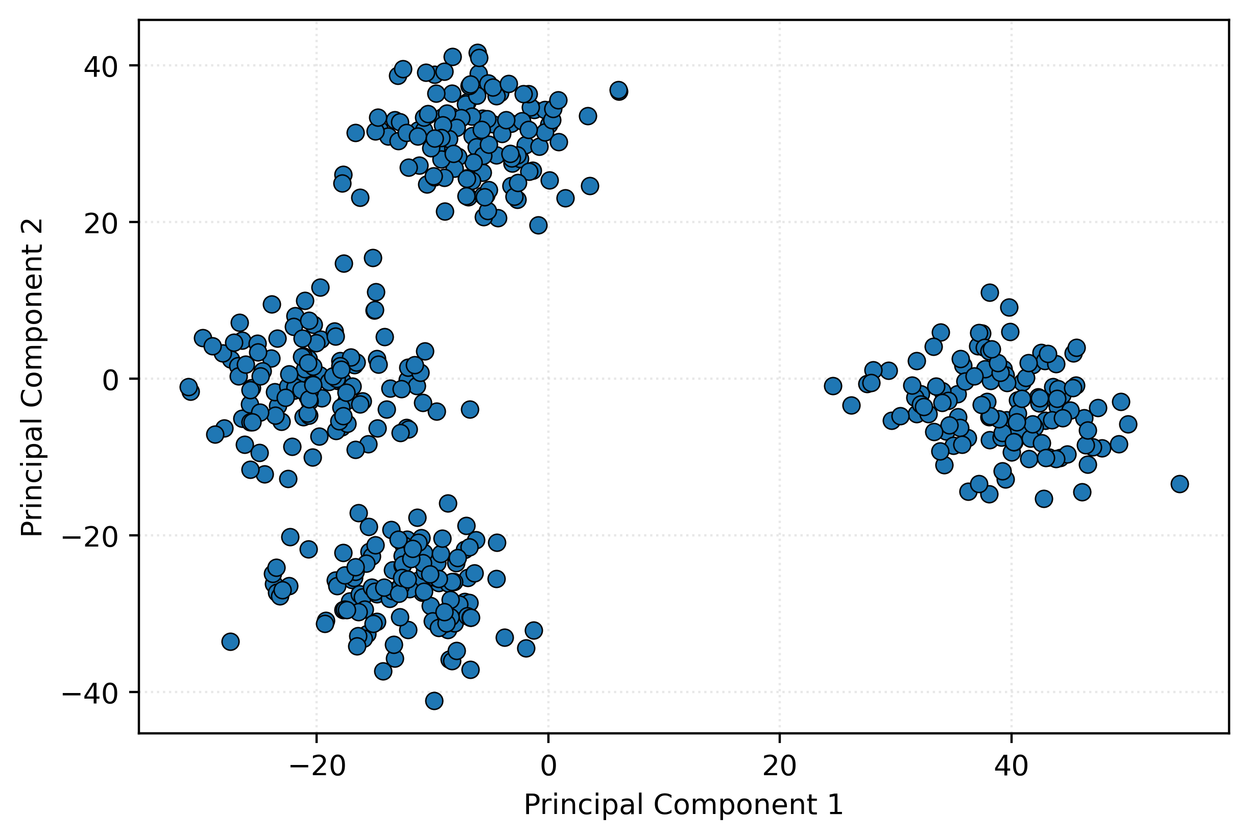
Well, would you look at that! With just two well-chosen features, we can detect an interesting structure in the data.
How does this work? In short, these two components are linear combinations of the original features. We’ll dive into PCA and related technique much later.
Anomaly Detection
The anomaly detection task seeks to identify samples that are significantly different from the majority of the data. These outliers or anomalies may represent errors, fraud, rare events, or other important deviations from normal patterns.
Potential examples include:
- Identifying network intrusions or cybersecurity threats from abnormal traffic behavior
- Finding defective products in manufacturing by spotting unusual sensor readings
- Monitoring patient health by detecting abnormal vital signs or test results
- Identifying equipment failures by recognizing unusual vibration or temperature patterns
Remember: In this situation, there is no response variable. We are detecting unusual samples only based on how they compare to other available data.
Let’s look at a sample of some example data:
| \(x_1\) | \(x_2\) |
|---|---|
| -0.79 | 10.14 |
| -6.00 | -7.42 |
| -1.32 | 7.65 |
| 1.54 | 1.84 |
| 6.44 | 1.36 |
| 5.89 | 0.69 |
| -4.03 | 9.49 |
| -5.99 | -7.34 |
| -4.50 | 9.31 |
| -9.05 | -10.18 |
Can you identify any samples that might be an anomaly just from looking at the numbers? It’s quite difficult without more context.
Let’s visualize this data:
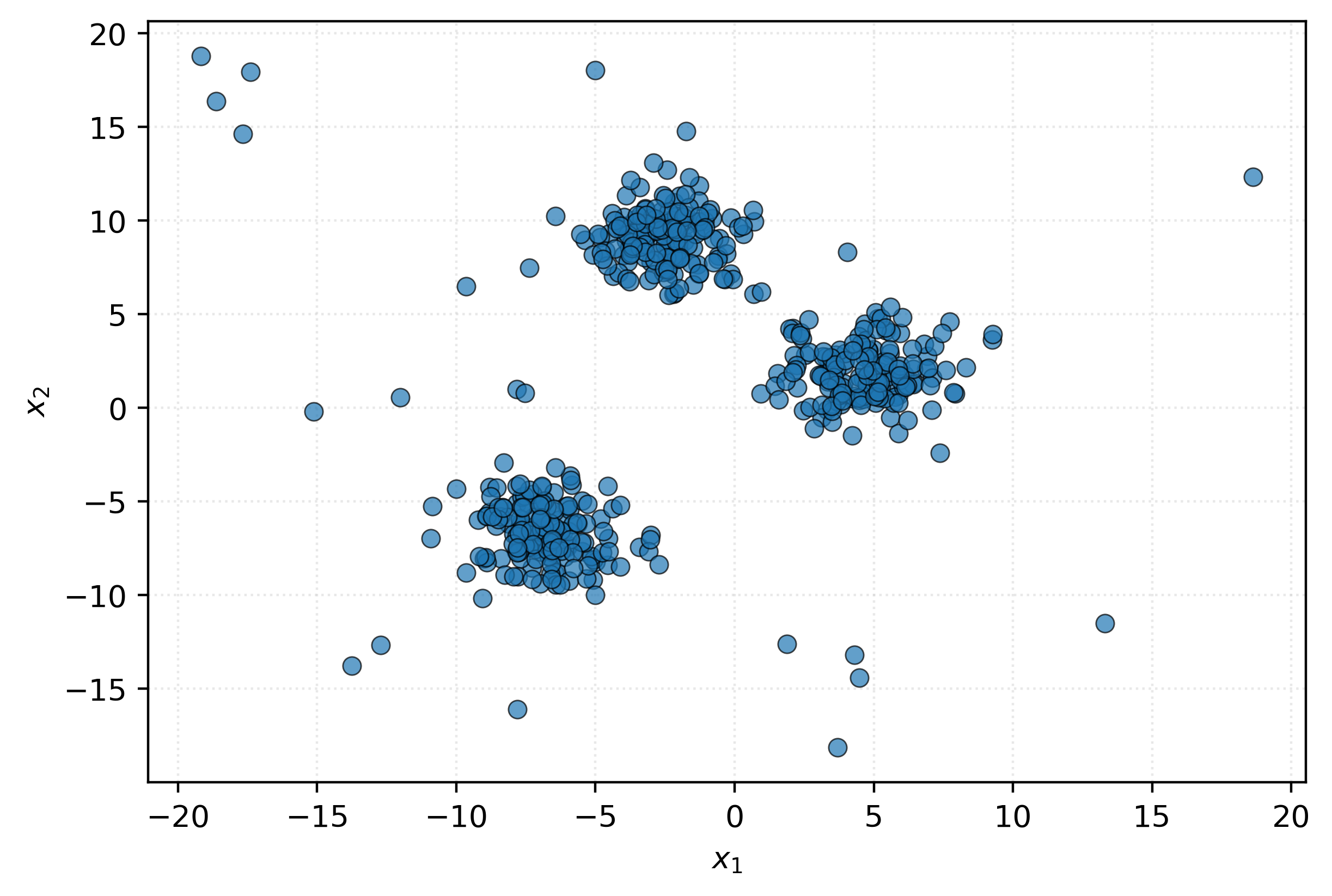
You can probably spot some potential outliers visually - the points that are far from the main “blobs” that emerge. Let’s apply an anomaly detection algorithm to identify these automatically and plot the results.
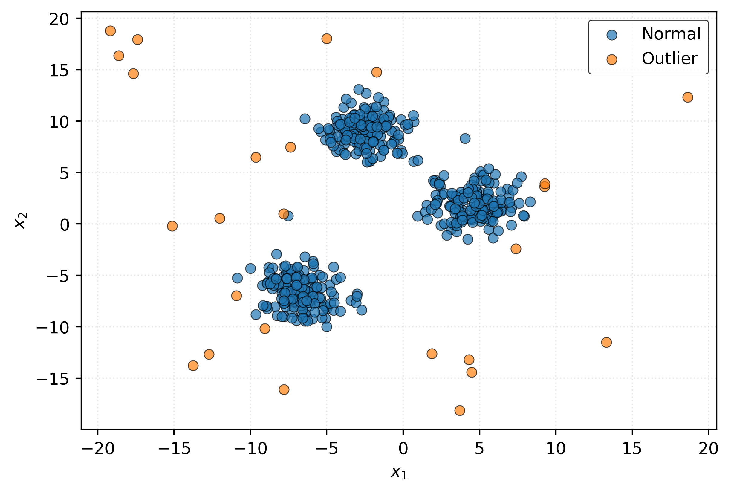
You might think that since we’ve detected these outliers, that we should remove them from the data. Much more on that later, but for now, a stern warning:

Density Estimation
The density estimation task seeks to understand the underlying probability distribution of the data. In a sense, this is the fundamental learning task. If we know the data distribution, we can answer essentially any questions about the data, without the need for any more statistics! Unfortunately, as we’ll learn, this is usually difficult-to-impossible. But in some situations, especially low-dimensional data, we can reasonably approximate true distributions.
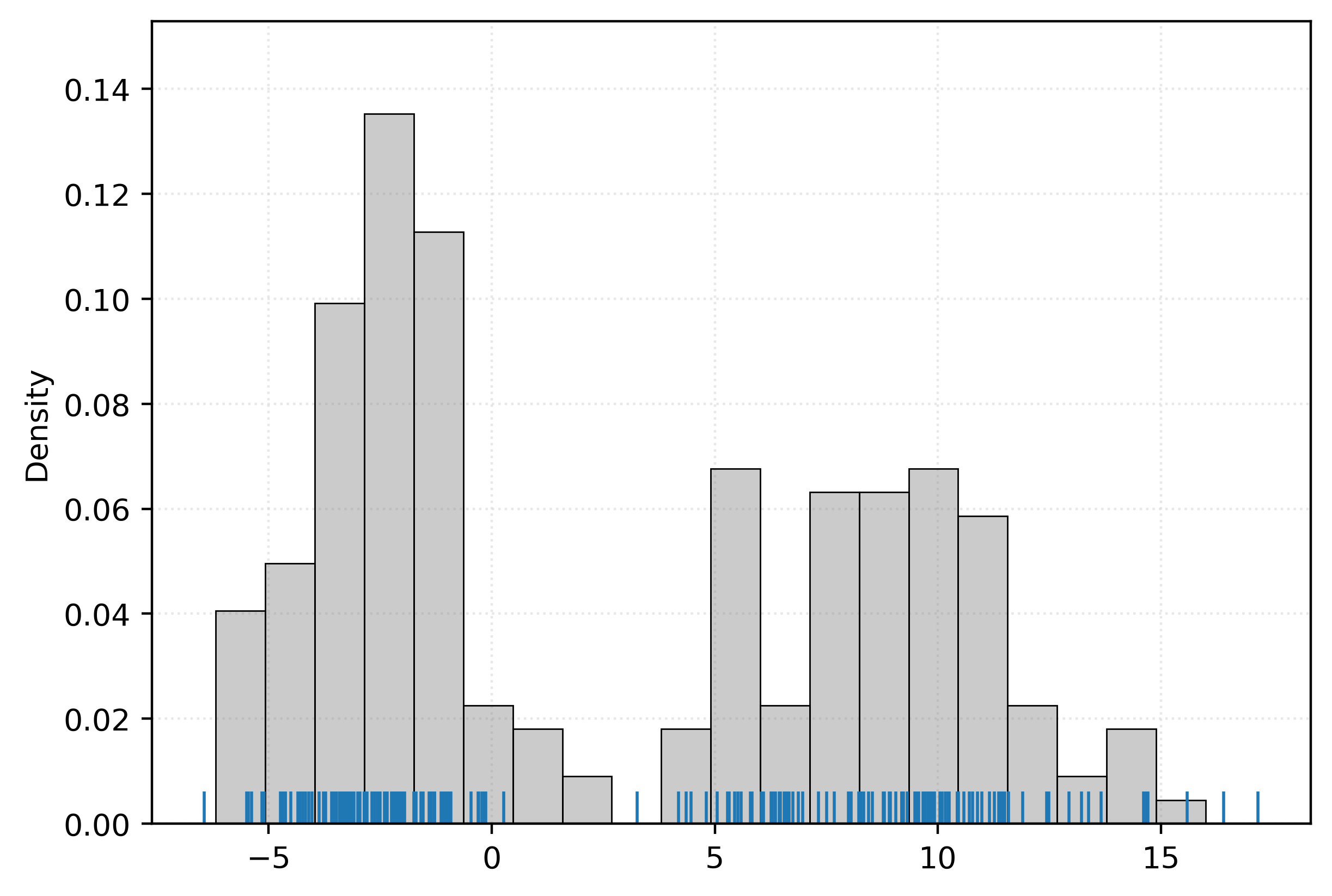
As an example, consider some one-dimensional data stored in a NumPy array.
[-2.84 -2.56 -2.07  6.75 11.58 10.7  -3.14 16.4  -2.21 -3.35  9.05 -3.48
 -2.95  8.34 -2.96 10.43  9.22 -4.63 -3.41 -1.28 -3.2   5.44 -3.23 -3.2
  6.87 -3.3  11.9   0.27 -2.41 -4.24  9.7   6.55 -2.68 -2.15 -2.38 -3.21
 -3.29 -2.97  5.05 11.38 -0.29 10.98 14.67 -3.87 -1.74  9.79 -0.16 -0.92
 -2.53 10.44  8.22 10.58 -3.59 14.61 -1.97 -2.25 10.46 -2.37 -2.86 -3.56
 -4.5   5.59  8.44 10.89 11.5   6.61 -2.2   5.28 -5.38 -6.44 11.16 -0.22
 -2.34 13.66 -2.86 -3.72  8.28  7.5  10.09 -3.26  5.3   4.19 -2.5  -3.21
  5.83 -1.28  9.48 -1.14 13.22 11.39 12.94 10.77 10.44  9.77  9.91  8.93
  8.05 -5.49 -3.41  8.8  10.25  6.09  8.78 17.17 10.17 -2.96 -1.97 -3.1
 -4.65 -1.97  5.32 -0.47  6.36 -4.17 -2.04  7.32  6.26  6.97 10.23 -2.36
 -5.15 11.27 -2.12 -4.34  9.19 -1.54  4.81  6.47  4.36  9.31 -3.33 -4.3
 12.44 -1.06 11.48  9.19 -0.31  6.35  6.29  9.54 15.59  9.92  7.67  6.44
 -1.59 -3.77  9.53 -1.99 -4.7   5.51  3.26 -1.36  8.53 -0.14  8.79  4.47
 -0.96  5.8   7.99 -1.11 -4.03 -0.2  -2.02 10.04 14.7  -1.05 10.05  6.04
 -1.29  9.66 -3.52 -2.02 -4.1  -1.   -2.86 -3.    9.79  8.91  9.57 11.36
 -1.7  -2.62 -2.85  9.84 -5.45 -2.01  6.66 -2.79 -5.1   9.71  9.89 -3.09
 -4.63 -1.95  6.57 -1.4  13.37 -4.73 11.45 12.49]
Let’s plot this data. Here we use both a histogram, as well as a rug plot.
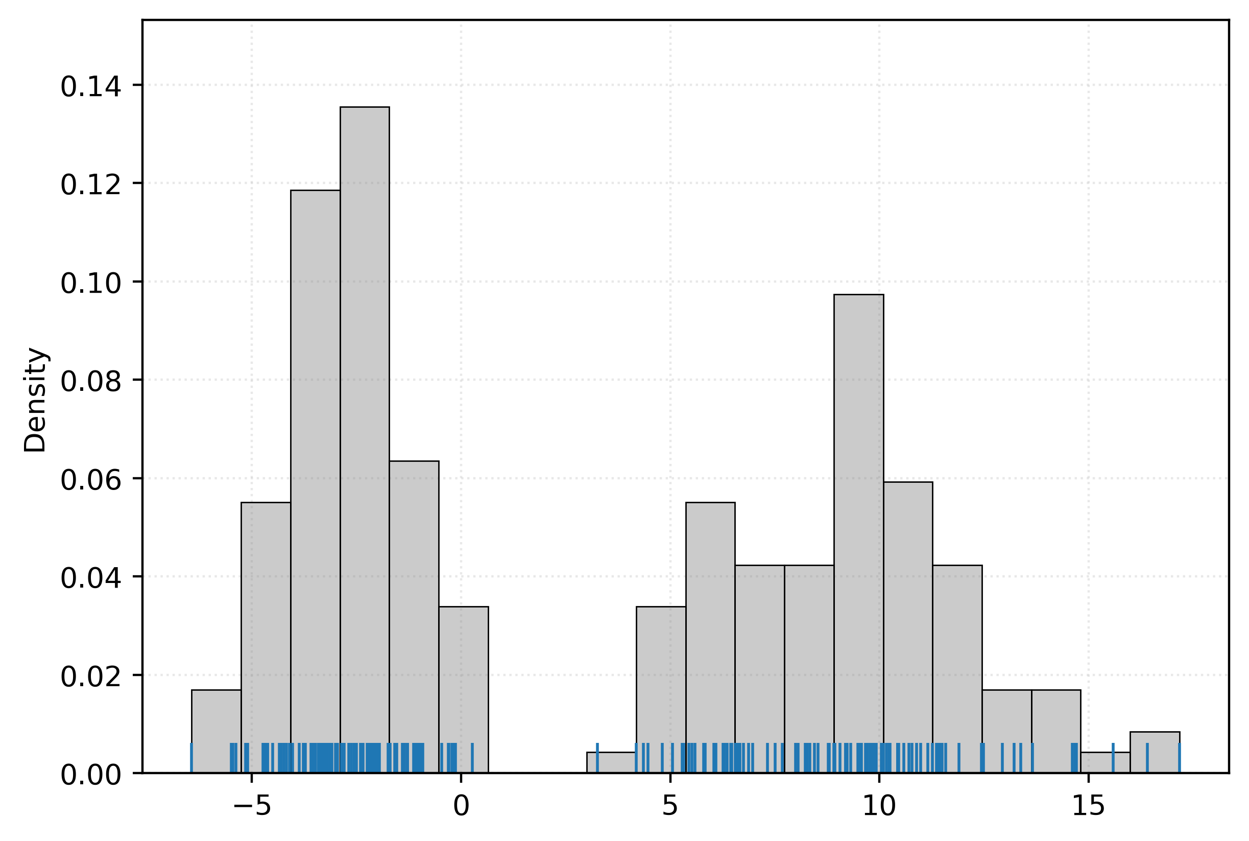
The rug plot is a method to visualize one-dimensional data along an axis. The histogram, is itself a form of density estimation!
Thought usually, when we want a density estimate, we’d like something smooth.
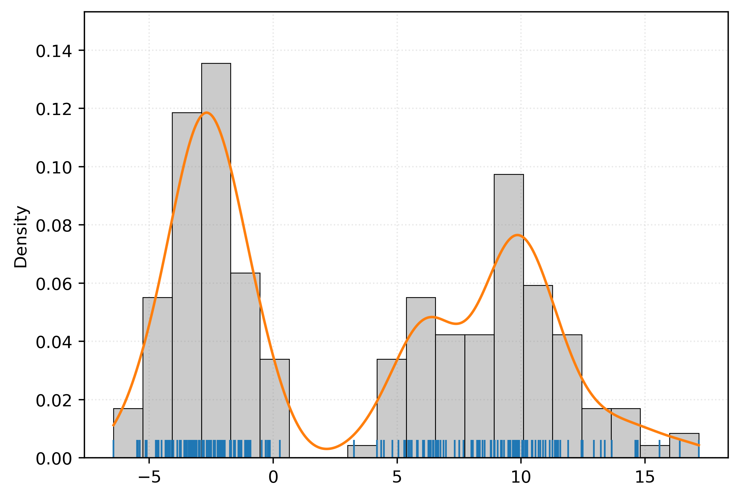
Here, we’ve add an estimated density that we obtained via a density estimation method.
With an estimated density, we can generate new data, that should seem as though it was sampled from the same distribution as the original data.
Is this data the same? Of course not. Does it seem reasonably similar to the original data? You betcha!5
Machine Learning Usage
In Chip Huyen’s Designing Machine Learning Systems, she summarizes what machine learning algorithms are generally designed to do.
Machine learning is an approach to (1) learn (2) complex patterns from (3) existing data and use these patterns to make (4) predictions on (5) unseen data.
- Learn – The system has the capacity to learn.
- Complex Patterns – There are patterns to learn, and they are complex.
- Existing Data – Data is available, or it’s possible to collect.
- Predictions – It’s a predictive problem.
- Unseen Data – Unseen data shares patterns with the training (existing) data.
We will largely think of these through the lens of supervised learning. In this context, when we say that the system can learn, we generally mean that there is some pattern or relationship (usually functional) between the target and the features, which we seek to learn. While we can of course learn simple patterns with machine learning, that is often unnecessary, and the trouble of using machine learning wouldn’t be worth the cost.
Because machine learning is a tool to learn from data, we of course need data in order to learn! In courses like CS 307, this fact can sometimes be undersold, as we will provide the data you work with. You don’t have to spend time and energy setting up systems to collect or generate data. But in the real world, they say that “data is the new oil” because data is what fuels machine learning. Do not underestimate the value of the data itself. Collecting or generating data can be a very non-trivial task.
For supervised learning, we of course need something (the response) to predict! Many supervised learning methods can be used to generally learn patterns and estimate a relationship between the response and the features. But in machine learning, the reason we do so is to make predictions, in particular on unseen data.
A subtle but important point is that the unseen data that we want to make predictions for, must have the same response-feature relationship for the model to work as expected. Of course, in practice we can never know with certainty that this is the case, but later, we’ll call out some heuristics to keep in mind when thinking about this necessity.
She continues and discusses situations where the use of machine learning algorithms truly shine. We’ll focus on two of these:
- It’s repetitive.
- The “cost” of incorrect predictions is cheap.
Machine learning, as the name suggests, is done by machines. Machines, unlike humans, have no issue repeating the same set of instructions over and over again.6 So, machine learning empowers us to make a lot of predictions. However, if we are making a lot of predictions, we are going to get some wrong. Your models will never be perfect. With that in mind, the “cost” (potential negative consequences, monetary or otherwise) had better not be too high. We will belabor this point throughout the course. When releasing a machine learning system into the world, you absolutely must consider the potential negative consequences.
Implicit in these points, is that feature data is cheap or easy to acquire, but the response data is expensive, difficult, potentially impossible to acquire. This difference is what makes prediction of the response useful; we can use the cheap features to predict the (otherwise expensive) response. Let’s tie some of these ideas together with two examples.
Example – Movie Recommendation System
Consider a streaming service trying to recommend movies to users. The features are easy to collect: user viewing history, movie genres, ratings, time of day, device type, etc. This information simply exists in a database somewhere, and it’s essentially automatically collected. However, getting the true response - whether a user will actually enjoy a specific movie - is expensive and difficult. You’d need to survey users after every viewing or wait for explicit ratings, which most users don’t provide.
The consequences of incorrect predictions are relatively low. If the system recommends a movie the user does not like, they simply don’t watch it, or stop watching early. This is a minimal cost, and potentially no cost if the user does not unsubscribe!
Example – Medical Diagnosis System
Consider instead, a system for diagnosing skin cancer from photos and patient information.7 Useful features in this situation include digital photos of the potentially problematic skin region and the patient’s age, skin cancer history, etc. These are all cheap to acquire. Digital photos are essentially free. However the response, whether a lesion is actually malignant, is anything but cheap. It can require pathology tests, biopsies, and of course, an expert dermatologist to visually inspect the skin and evaluate the test results. Doctors’ time is not cheap!
The consequences of incorrect predictions from a machine learning algorithm here are extremely high. The stakes are potentially life-and-death. A false negative, failing to detect a cancer when it exists, could quite literally result in death. But false negatives are not the only potential mistake! A false positive, incorrectly detecting cancer when it does not exist, also has negative (but lesser) consequences. Incorrectly detecting cancer could lead to unnecessary anxiety, additional procedures, and increased medical bills.
Much later, we will discuss the tradeoff between false negatives and false positives in detail.
Footnotes
Using “predictors” for inputs would quickly become confusing given that prediction is such a core concept in machine learning. “Independent” and “dependant” variables are simply confusion terminology as independent has a very specific meaning in statistics and machine learning.↩︎
Probably something like \(\sin(-2.25)\).↩︎
Defining Modern NBA Player Positions - Applying Machine Learning to Uncover Functional Roles in Basketball↩︎
“You betcha!” is Midwestern for “yes, absolutely” but enthusiastically.↩︎
This is essentially the reason the field of computing exists.↩︎
This is such a common task that there are review papers on the subject, for example: AI-Powered Diagnosis of Skin Cancer: A Contemporary Review, Open Challenges and Future Research Directions.↩︎