# basic imports
import numpy as np
import pandas as pd
import seaborn as sns
import matplotlib.pyplot as plt

# model imports
from sklearn.neighbors import KNeighborsRegressor
from sklearn.tree import DecisionTreeRegressor

# metric imports
from sklearn.metrics import root_mean_squared_error

# model selection imports
from sklearn.model_selection import train_test_split

# data imports
from sklearn.datasets import make_friedman1Generalization
Model Flexibility, Overfitting, and the Bias-Variance Tradeoff
Objectives
In this note, we will discuss:
- model flexibility and its relationship to model performance and generalization,
- overfitting and underfitting as fundamental problems in machine learning,
- and the bias-variance tradeoff as a theoretical framework for understanding generalization.
Along the way, we will briefly introduce decision trees then use our understanding of model flexibility to explore how decision tree parameters relate to model flexibility.
Python Setup
Notebook
The following Jupyter notebook contains some starter code that may be useful for following along with this note.
Model Flexibility
A model’s flexibility determines how well the model can learn the training data.
- A “flexible” model can learn “complex” patterns in the data, but is also more likely to overfit.
- An “inflexible” model is less likely to overfit, but may not be able to learn the true underlying patterns in the data.
Given a particular dataset, when fitting a model, you are essentially trying to find a model that is flexible enough to learn the underlying patterns in the data, but not so flexible that it learns the noise in the data.
How do we control a model’s flexibility? Our main tool for controlling a model’s flexibility are its tuning parameters, which may also be called hyperparameters.
Let’s investigate with \(k\) for \(k\)-nearest neighbors.
# simulate data
X, y = make_friedman1(
    n_samples=1000,
    noise=0.5,
    random_state=42,
)
# split the data
X_train, X_test, y_train, y_test = train_test_split(
X,
y,
test_size=0.25,
random_state=42,
)# define range of k values to search over
k_values = range(1, 152, 2)# initialize storage for train RMSE values
train_rmse = []
# initialize storage for test RMSE values
test_rmse = []# fit models and calculate train and test RMSE for each value of k
for k in k_values:
# initialize model, with the current k
knn = KNeighborsRegressor(n_neighbors=k)
# fit the model to the (validation) train data
knn.fit(X_train, y_train)
# get train predictions
y_train_pred = knn.predict(X_train)
# calculate (and store) train RMSE
train_rmse.append(root_mean_squared_error(y_train, y_train_pred))
# get test predictions
y_test_pred = knn.predict(X_test)
# calculate (and store) test RMSE
test_rmse.append(root_mean_squared_error(y_test, y_test_pred))Show Code for Plot
fig, ax = plt.subplots(figsize=(10, 6))
ax.plot(k_values, train_rmse, marker="o", markersize=5, label="Train RMSE")
ax.plot(k_values, test_rmse, marker="o", markersize=5, label="Test RMSE")
ax.set_xlabel("k")
ax.set_ylabel("RMSE")
ax.legend()
plt.show()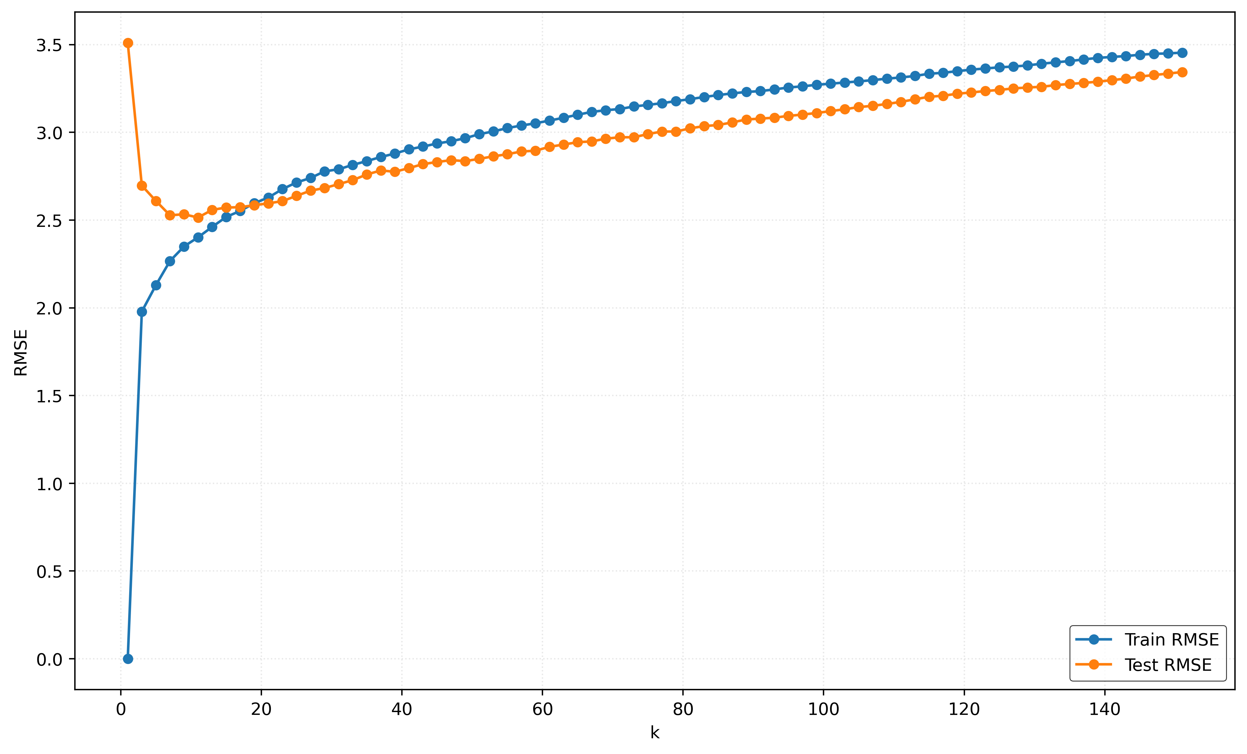
How does \(k\) relate to model flexibility?
- A small \(k\) has low train error, thus is more flexible model.
- A large \(k\) has high train error, thus is a less flexible model.
That is, as \(k\) increases, the model becomes less flexible.
How do we know this? Note that as \(k\) increases, the train RMSE increases. Said in reverse, as \(k\) decreases, the train RMSE decreases, and thus the model better learns the training data.
Overfitting
What is overfitting?
As the name subtly suggests, overfitting occurs when a model has learned too much. That is, it learned too much of the data, and has overfit to a particular dataset. In particular, it has learned the training data so well, that beyond learning the underlying patterns in the data, it has also learned the noise in the data.
How do we know when overfitting has occurred?
- The model has a low train error, relative to training error for other models.
- The model has a high test error, relative to test error for other models.
In other words, overfitting occurs when a model is too flexible for a particular dataset.
Overfitting is one of two problems that we will encounter related to model flexibility. The other and opposite problem is that of underfitting.
How do we know when underfitting has occurred?
- The model has a high train error, relative to training error for other models.
- The model has a high test error, relative to test error for other models.
In other words, underfitting occurs when a model is not flexible enough for a particular dataset.
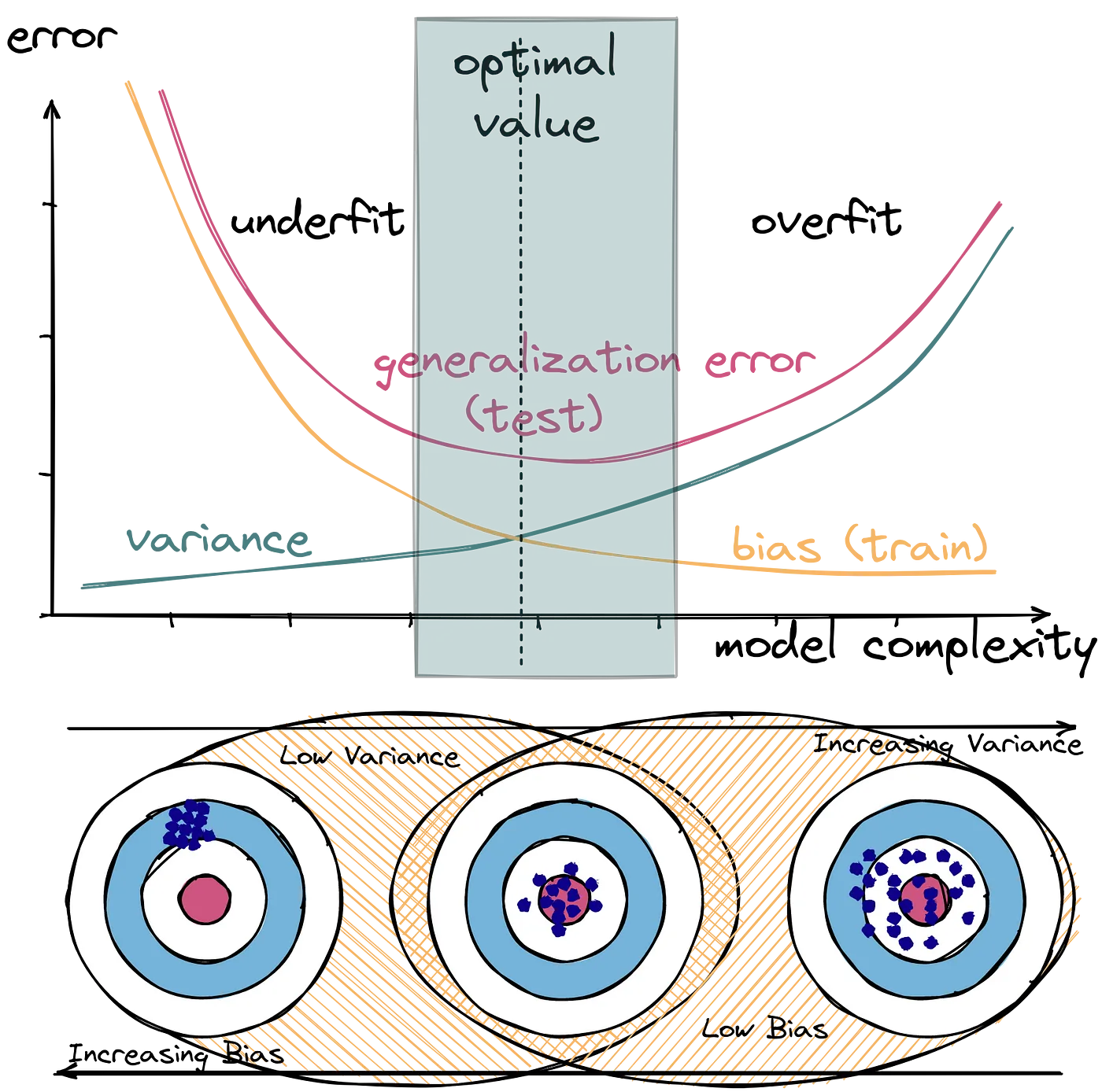
We can summarize these definitions graphically, as we have done in Figure 2.
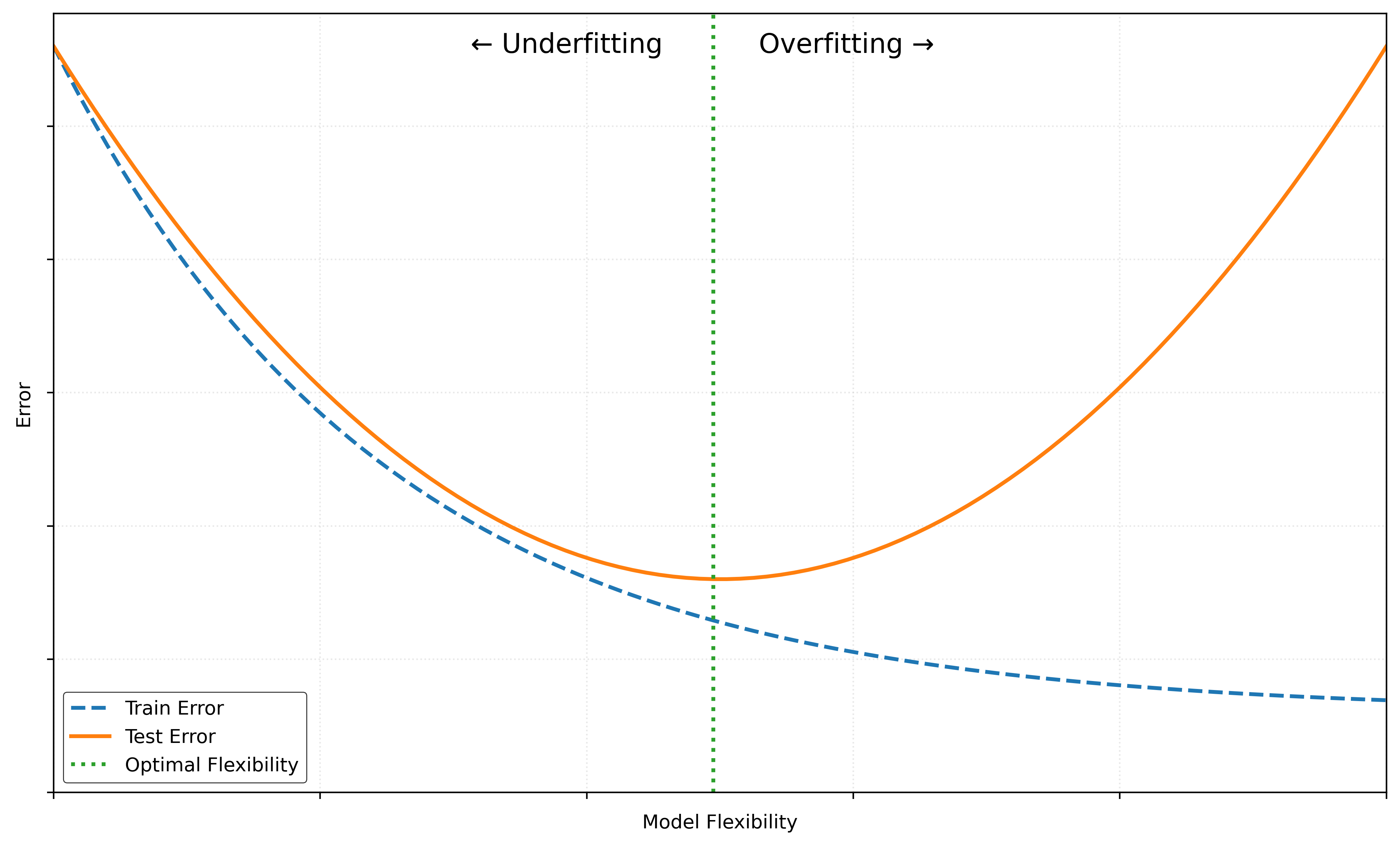
Be aware, Figure 2 is highly idealized. In practice, the U-shaped curve may not be so smooth, or even U-shaped at all!
Example: Decision Tree Tuning Parameters
# define range of depth values to search over
max_depths = range(1, 42, 1)
# initialize storage for train RMSE values
train_rmse = []
# initialize storage for test RMSE values
test_rmse = []# fit models and calculate train and test RMSE for each value of the tuning parameter
for depth in max_depths:
# initialize model, with the current k
tree = DecisionTreeRegressor(max_depth=depth)
# fit the model to the (validation) train data
tree.fit(X_train, y_train)
# get train predictions
y_train_pred = tree.predict(X_train)
# calculate (and store) train RMSE
train_rmse.append(root_mean_squared_error(y_train, y_train_pred))
# get test predictions
y_test_pred = tree.predict(X_test)
# calculate (and store) test RMSE
test_rmse.append(root_mean_squared_error(y_test, y_test_pred))Show Code for Plot
fig, ax = plt.subplots(figsize=(10, 6))
ax.plot(max_depths, train_rmse, marker="o", markersize=5, label="Train RMSE")
ax.plot(max_depths, test_rmse, marker="o", markersize=5, label="Test RMSE")
ax.set_xlabel("Maximum Depth")
ax.set_ylabel("RMSE")
ax.legend()
plt.show()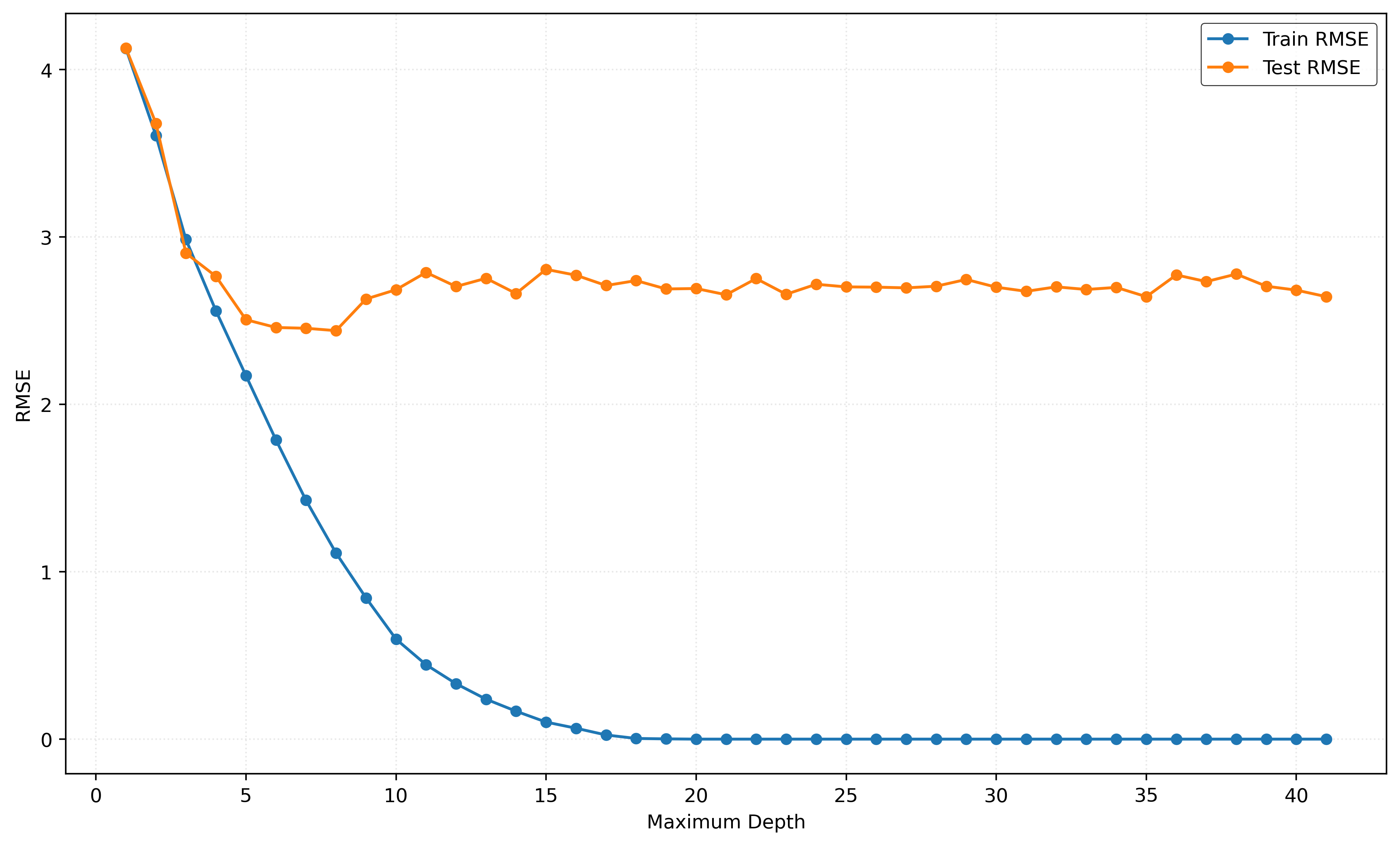
# define range of min-split values to search over
min_samples_split = range(2, 101, 2)
# initialize storage for train RMSE values
train_rmse = []
# initialize storage for test RMSE values
test_rmse = []# fit models and calculate train and test RMSE for each value of the tuning parameter
for minimum in min_samples_split:
# initialize model, with the current k
tree = DecisionTreeRegressor(min_samples_split=minimum)
# fit the model to the (validation) train data
tree.fit(X_train, y_train)
# get train predictions
y_train_pred = tree.predict(X_train)
# calculate (and store) train RMSE
train_rmse.append(root_mean_squared_error(y_train, y_train_pred))
# get test predictions
y_test_pred = tree.predict(X_test)
# calculate (and store) test RMSE
test_rmse.append(root_mean_squared_error(y_test, y_test_pred))Show Code for Plot
fig, ax = plt.subplots(figsize=(10, 6))
ax.plot(min_samples_split, train_rmse, marker="o", markersize=5, label="Train RMSE")
ax.plot(min_samples_split, test_rmse, marker="o", markersize=5, label="Test RMSE")
ax.set_xlabel("Minimum Samples to Split")
ax.set_ylabel("RMSE")
ax.legend()
plt.show()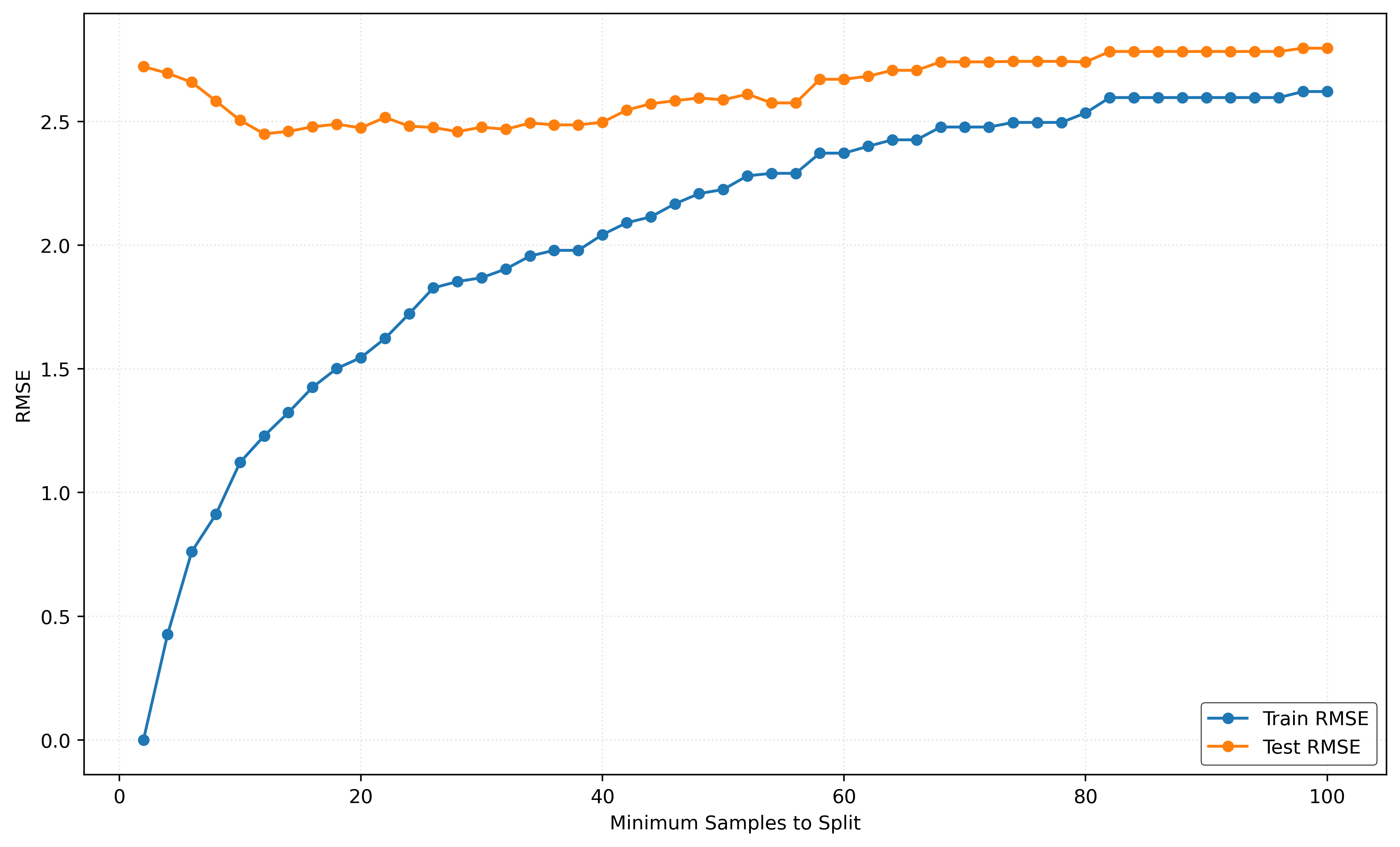
Bias and Variance of Estimators
So three statisticians go deer hunting.
The first one misses ten feet to the left.
Second misses ten feet to the right.
The third one jumps up and down and says, “I hit it!”
– As told by Samuel Norman Seaborn, The West Wing, Season 3 Episode 08
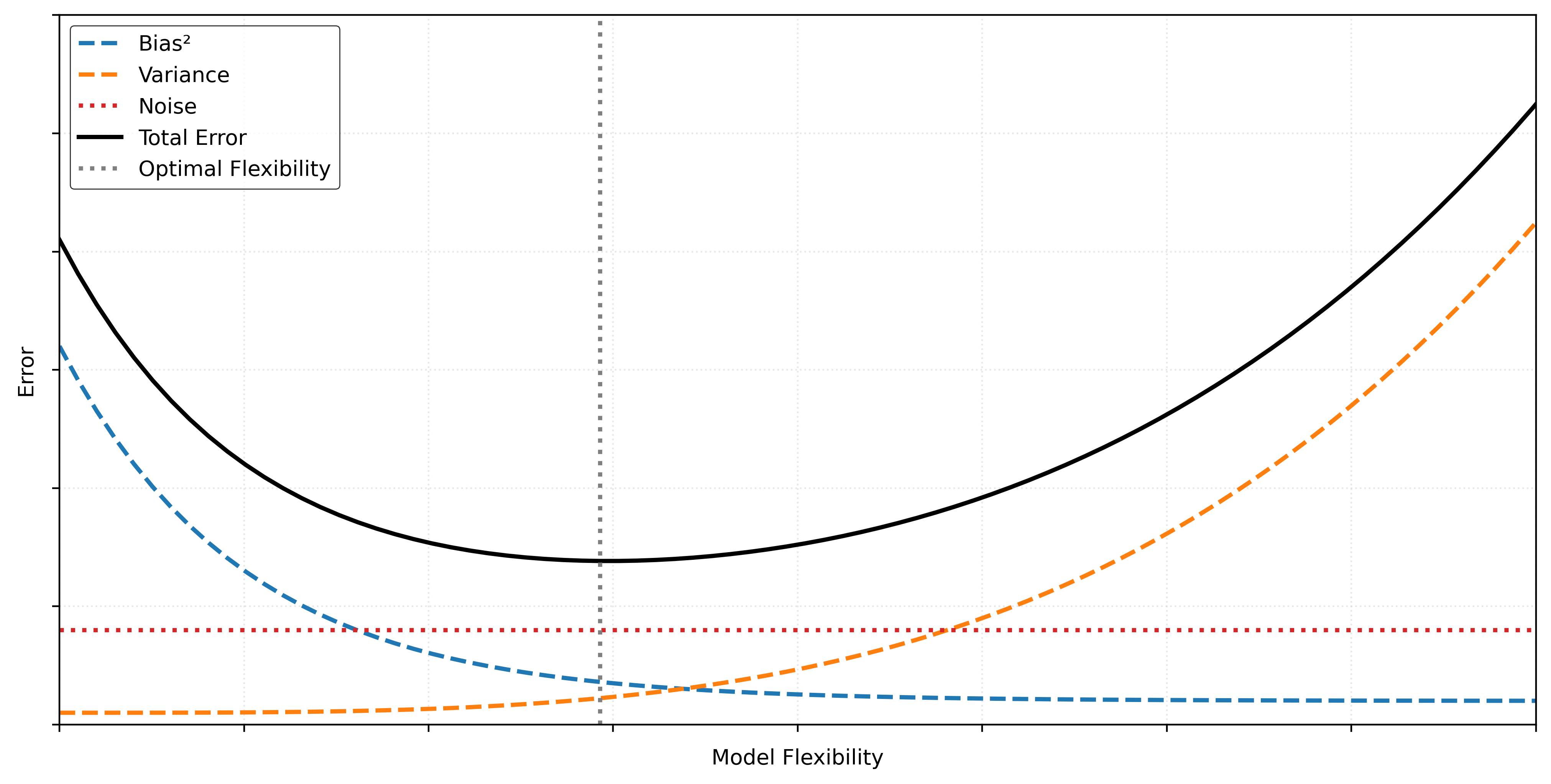
Bias-Variance Tradeoff
There are three sources of error in a model for supervised learning:
- Bias
- Variance
- Noise
The bias and variance together make up the reducible error in a model. By selecting a model of an appropriate flexibility, we can, as the name suggests, reduce this error. The noise is also called the irreducible error.
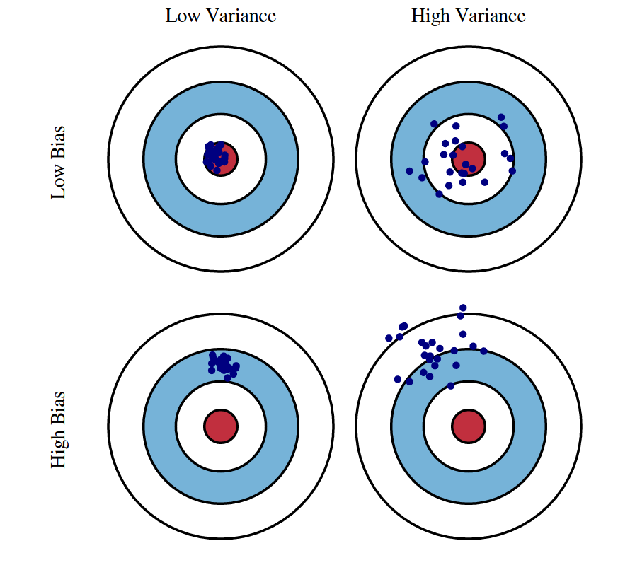
The bias of a model is the error due to the model’s assumptions or lack of flexibility. It is systematic error due to the model’s inability to (fully) learn the true underlying patterns in the data.
The variance of a model is the error due to the model’s sensitivity to the training data. It is the error due to the model (partially) learning some noise in the training data. The model changes (too much) if the training data is changed.
Both bias and variance are related to the model’s flexibility.
- As flexibility increases, bias decreases.
- As flexibility increases, variance increases.
We can summarize these definitions graphically, as we have done in Figure 6.
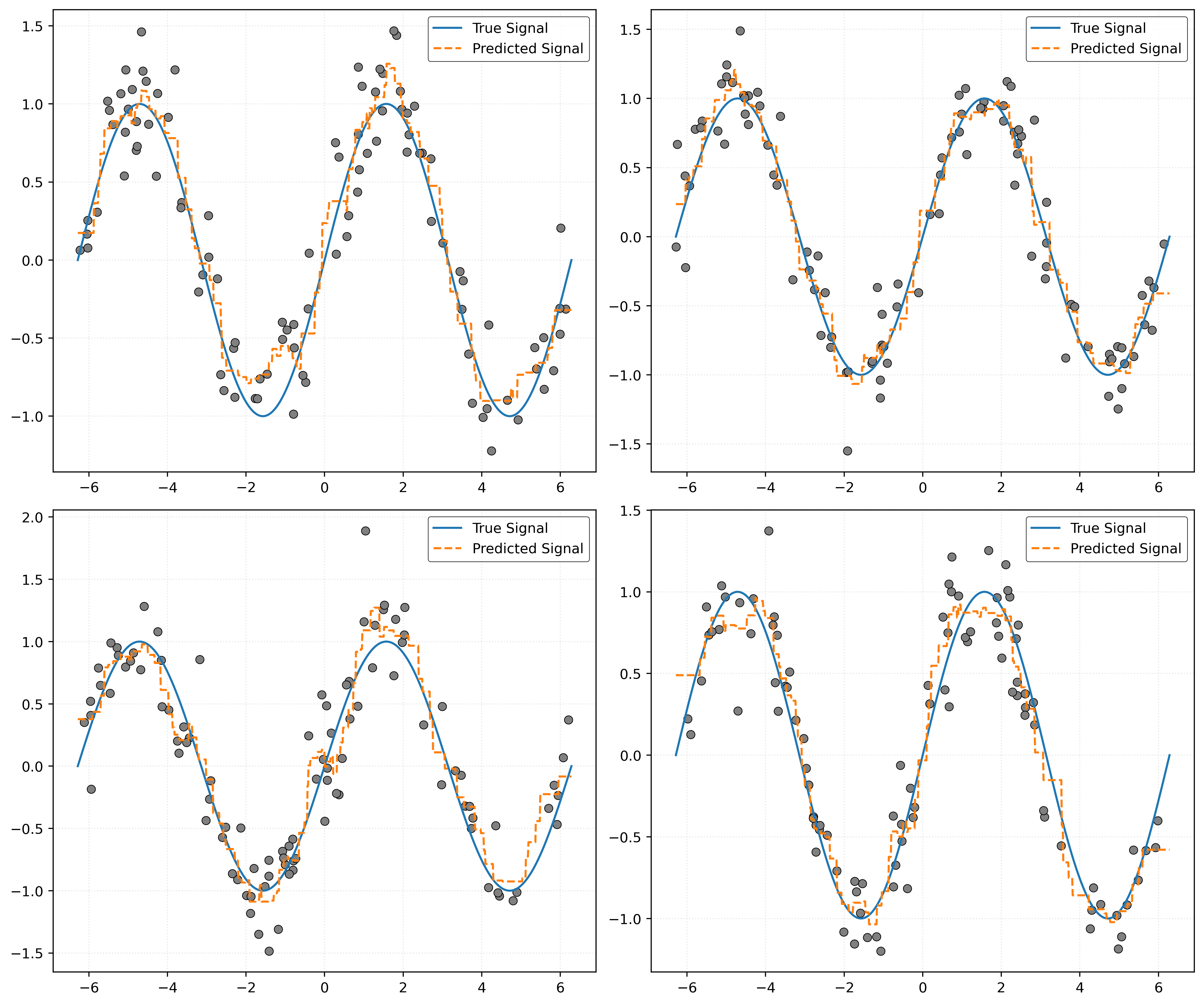
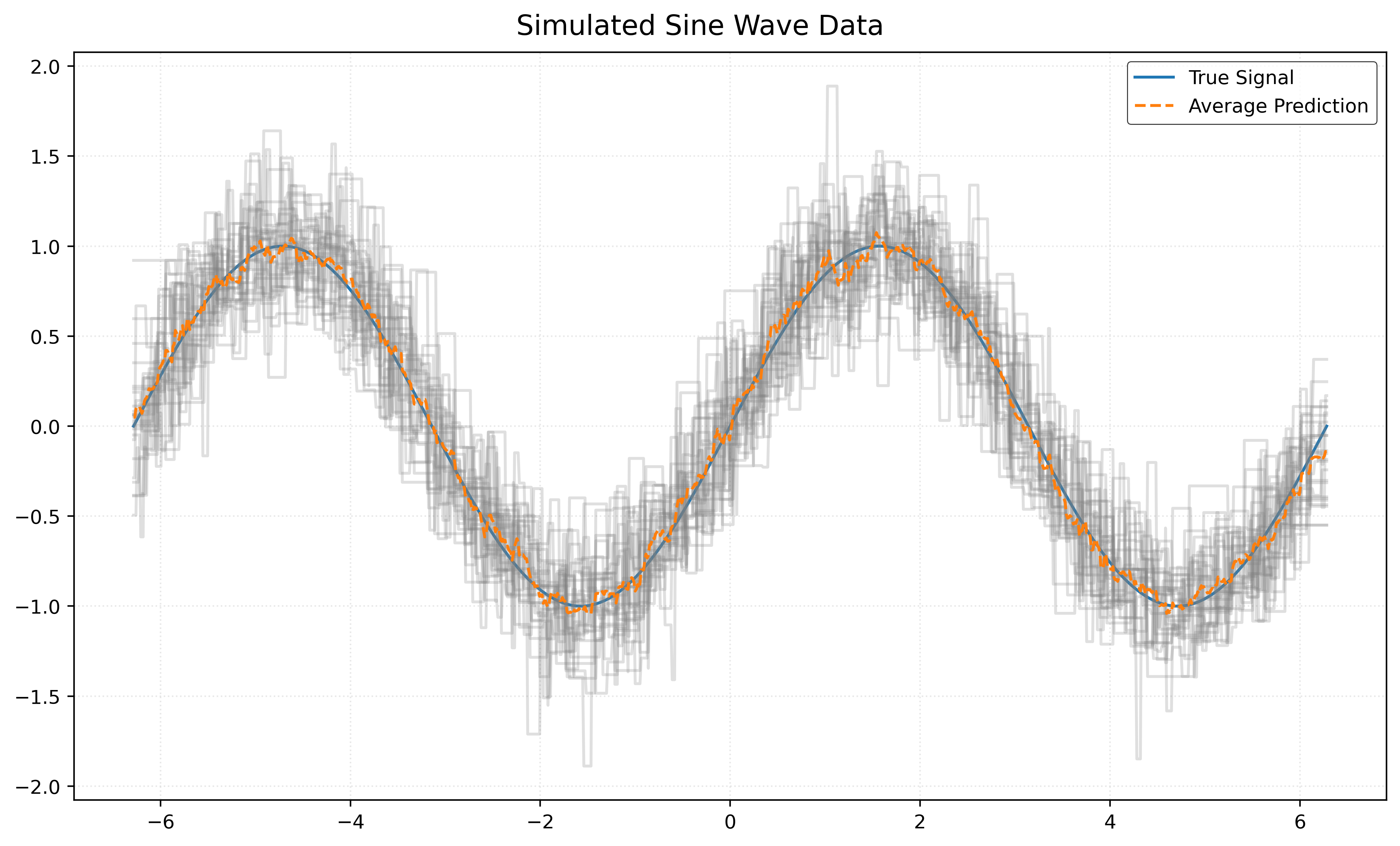
Example: Bias-Variance Tradeoff in KNN
Let’s return to our usual simulated sine wave example.
def simulate_sin_data(n, sd, seed):
    np.random.seed(seed)
    X = np.random.uniform(
        low=-2 * np.pi,
        high=2 * np.pi,
        size=(n, 1),
    )
    signal = np.sin(X).ravel()
    noise = np.random.normal(
        loc=0,
        scale=sd,
        size=n,
    )
    y = signal + noise
    return X, y
Let’s investigate the bias and variance of KNN models as a function of potential values of \(k\).
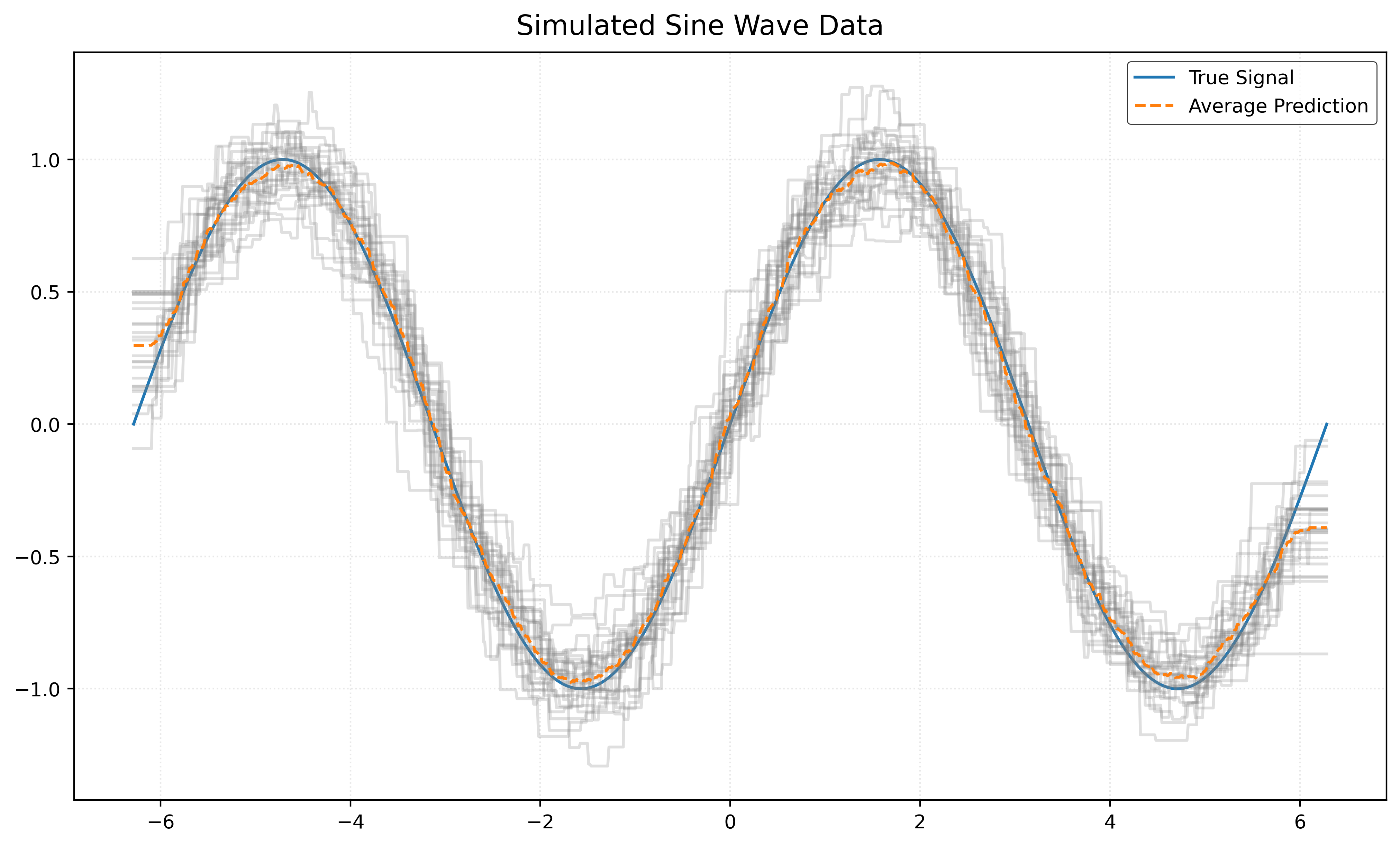
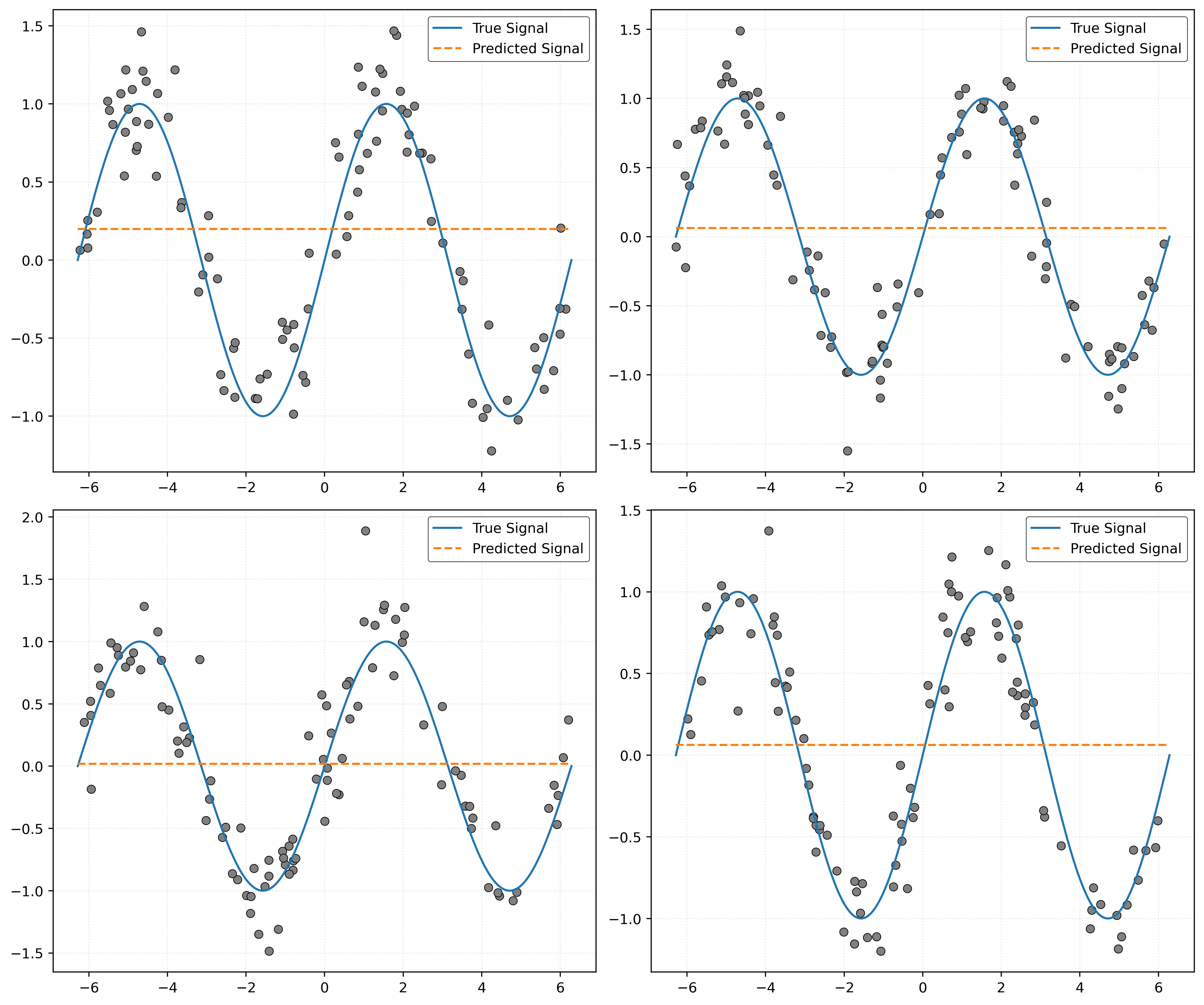
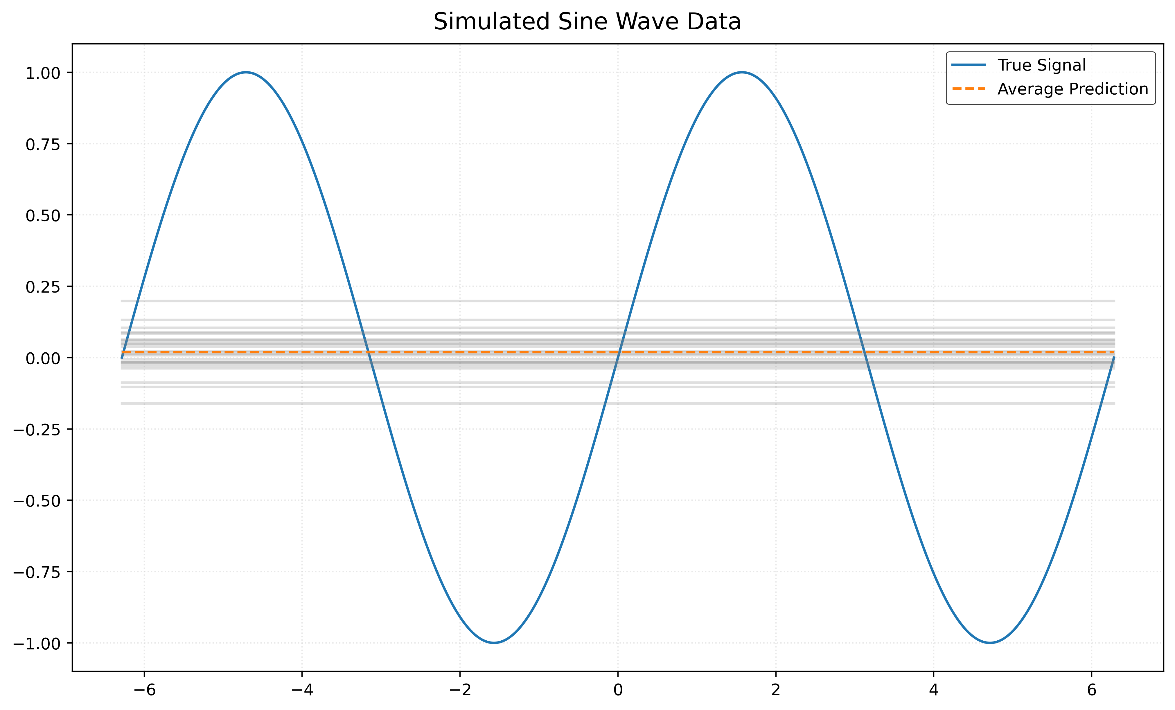
Bias and Variance with \(k = 100\)
First, consider \(k = 100\). To investigate bias and variance, we will need to repeatedly simulate data, then each time fit a model with \(k = 100\).
Bias and Variance with \(k = 1\)
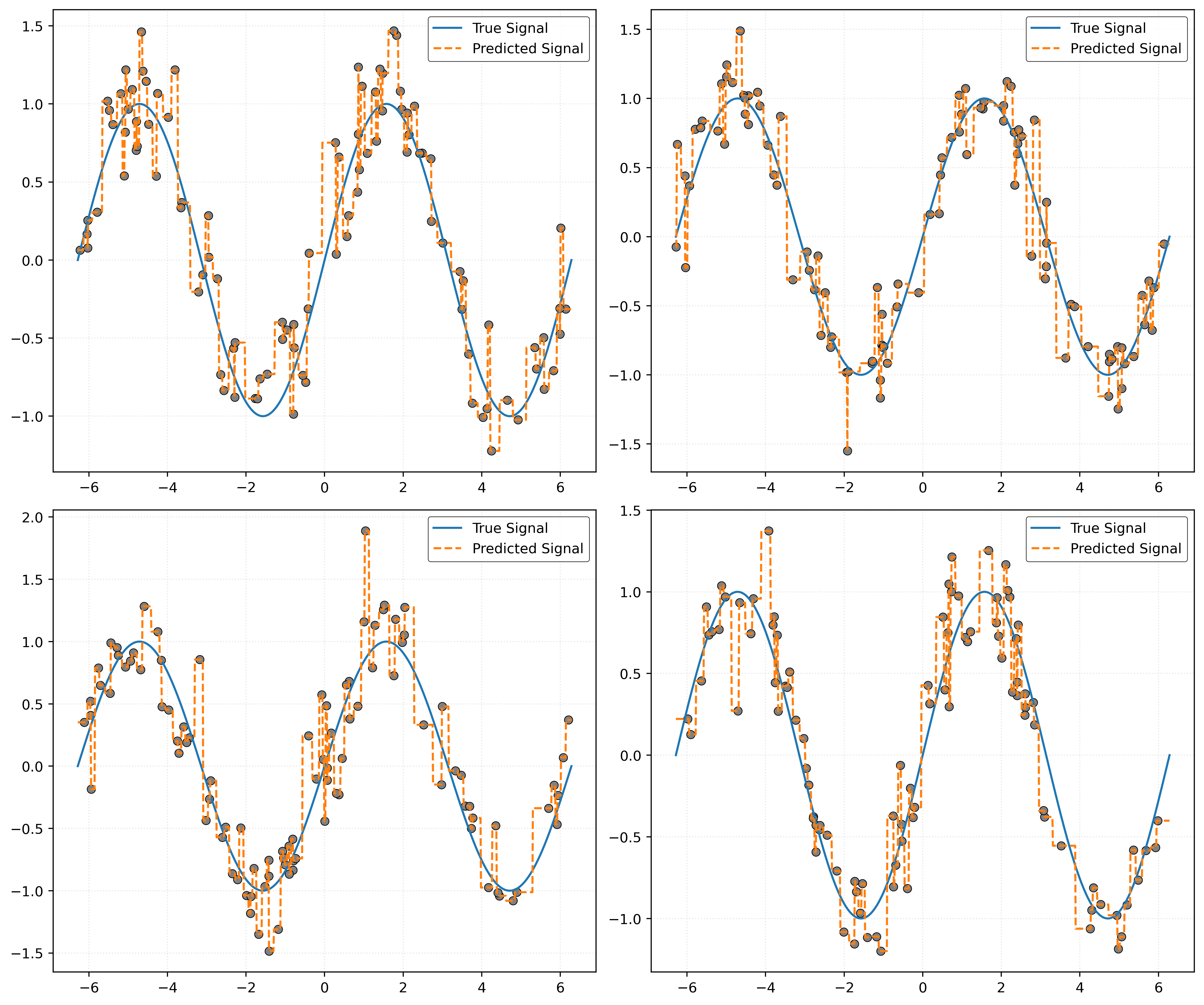
Bias and Variance with \(k = 5\)