Cross-Validation

Tuning with Resampling

Table of Contents

• Objectives
• Python Setup
• Notebook
• Validation and Test Data
  • Correct Approach: Validation and Test Data
  • Optimistic Approach: Test Data Only
• Cross-Validation
  • Tuning with Single Validation Set
  • Tuning with Cross-Validation
• Grid Search
• Example: Palmer Penguins

Objectives

In this note, we will discuss:

• the need for both validation and test sets,
• cross-validation,
• and grid search for parameter tuning.

We will conclude with an example that applies cross-validation and a grid search to the Palmer penguins data.

Python Setup

# basic imports
import numpy as np
import pandas as pd
import seaborn as sns
import matplotlib.pyplot as plt
from pprint import pprint

# model imports
from sklearn.neighbors import KNeighborsRegressor
from sklearn.neighbors import KNeighborsClassifier

# metric imports
from sklearn.metrics import root_mean_squared_error
from sklearn.metrics import accuracy_score

# model selection imports
from sklearn.model_selection import train_test_split
from sklearn.model_selection import KFold
from sklearn.model_selection import cross_val_score
from sklearn.model_selection import GridSearchCV

# preprocessing imports
from sklearn.preprocessing import StandardScaler
from sklearn.preprocessing import OneHotEncoder
from sklearn.impute import SimpleImputer
from sklearn.compose import ColumnTransformer
from sklearn.pipeline import Pipeline

# data imports
from palmerpenguins import load_penguins

Notebook

The following Jupyter notebook contains some starter code that may be useful for following along with this note.

• Cross-Validation Notebook

Validation and Test Data

Before introducing cross-validation, you might still be wondering: Why do we need both a validation set and a test set? Why not just a test set? That certainly would be easier!

• The validation set is used to select a model, through hyperparameter tuning.
• The test set is used to evaluate the model.

But again, why can’t the test set be used to select and evaluate a model? Aren’t we evaluating the model when we select it? Indeed we are, but that evaluation is only used for selection. The evaluation performed using the test data is the final evaluation of the model, which gives an estimate of how the model will perform on new, unseen data.

When we use the validation data to select a model, we are “seeing” or “looking” at that data, despite not fitting the model with that data.

Using only a test set for both selection and evaluation would lead to an optimistic estimate of the model’s performance.

The following simulations studies demonstrate the optimistic bias that results from using the test set for both selection and evaluation.

def simulate_sin_data(n, sd, seed):
    np.random.seed(seed)
    X = np.random.uniform(low=-2 * np.pi, high=2 * np.pi, size=(n, 1))
    signal = np.sin(X).ravel()
    noise = np.random.normal(loc=0, scale=sd, size=n)
    y = signal + noise
    return X, y

k_values = np.arange(1, 20, 2)

Correct Approach: Validation and Test Data

rmse_tests = []
rmse_trues = []

for sim in range(250):

    # simulate data
    X, y = simulate_sin_data(n=500, sd=0.25, seed=sim)

    # train-test split data
    X_train, X_test, y_train, y_test = train_test_split(
        X,
        y,
        test_size=0.20,
        random_state=42,
    )

    # train-validate split the data
    X_vtrain, X_validation, y_vtrain, y_validation = train_test_split(
        X_train,
        y_train,
        test_size=0.20,
        random_state=42,
    )

    # initalize list to store validation rmse values
    rmse_val = []


    for k in k_values:
        knn = KNeighborsRegressor(n_neighbors=k)
        knn.fit(X_vtrain, y_vtrain)
        y_pred = knn.predict(X_validation)
        validation_rmse = root_mean_squared_error(y_validation, y_pred)
        rmse_val.append(validation_rmse)

    # "select" model with best k
    best_k = k_values[np.argmin(rmse_val)]

    # refit model to full train data with chosen k
    knn = KNeighborsRegressor(n_neighbors=best_k)
    knn.fit(X_train, y_train)

    # calculate and store test rmse
    test_rmse = root_mean_squared_error(y_test, knn.predict(X_test))
    rmse_tests.append(test_rmse)

    # simulate a lot of "new" and "unseen" data
    X_new, y_new = simulate_sin_data(
        n=10000,
        sd=0.25,
        seed=42,
    )

    # calculate and store the "true" rmse
    rmse_true = root_mean_squared_error(y_new, knn.predict(X_new))
    rmse_trues.append(rmse_true)

ratios = np.array(rmse_tests) / np.array(rmse_trues)
print(np.mean(ratios))
print(np.mean(ratios < 1))

0.9887479393487324
0.58

fig, ax = plt.subplots()
ax.hist(ratios, bins=30, edgecolor="black")
ax.set_xlabel("RMSE Ratio: Estimated vs True")
ax.set_ylabel("Frequency")
plt.show()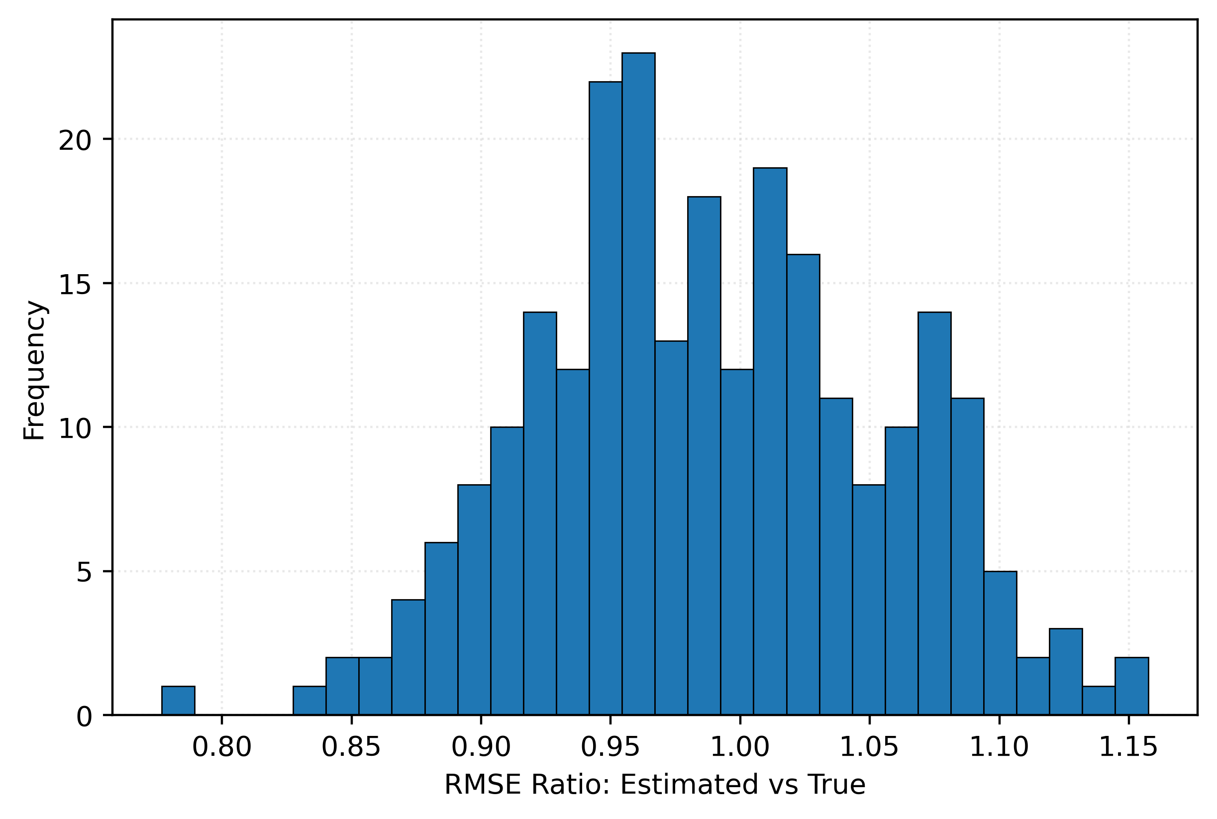

Figure 1: A histogram of the ratios of the estimated versus true RMSE values calculated via a simulation study that used a validation set for selection and a separate test set for evaluation.

Optimistic Approach: Test Data Only

rmse_tests = []
rmse_trues = []

for sim in range(250):

    # simulate data
    X, y = simulate_sin_data(n=500, sd=0.25, seed=sim)

    # train-test split data
    X_train, X_test, y_train, y_test = train_test_split(
        X,
        y,
        test_size=0.20,
        random_state=42,
    )

    # initalize list to store "validation" rmse values
    rmse_val = []

    # calculate "validation" rmse for each k
    for k in k_values:
        knn = KNeighborsRegressor(n_neighbors=k)
        knn.fit(X_train, y_train)
        y_pred = knn.predict(X_test)
        validation_rmse = root_mean_squared_error(y_test, y_pred)
        rmse_val.append(validation_rmse)

    # "select" model with best k
    best_k = k_values[np.argmin(rmse_val)]

    # refit model to full train data with chosen k
    knn = KNeighborsRegressor(n_neighbors=best_k)
    knn.fit(X_train, y_train)

    # calculate and store test rmse
    test_rmse = root_mean_squared_error(y_test, knn.predict(X_test))
    rmse_tests.append(test_rmse)

    # simulate a lot of "new" and "unseen" data
    X_new, y_new = simulate_sin_data(
        n=10000,
        sd=0.25,
        seed=42,
    )

    # calculate and store the "true" rmse
    rmse_true = root_mean_squared_error(y_new, knn.predict(X_new))
    rmse_trues.append(rmse_true)

ratios = np.array(rmse_tests) / np.array(rmse_trues)
print(np.mean(ratios))
print(np.mean(ratios < 1))

0.9702873893641341
0.688

fig, ax = plt.subplots()
ax.hist(ratios, bins=30, edgecolor="black")
ax.set_xlabel("RMSE Ratio: Estimated vs True")
ax.set_ylabel("Frequency")
plt.show()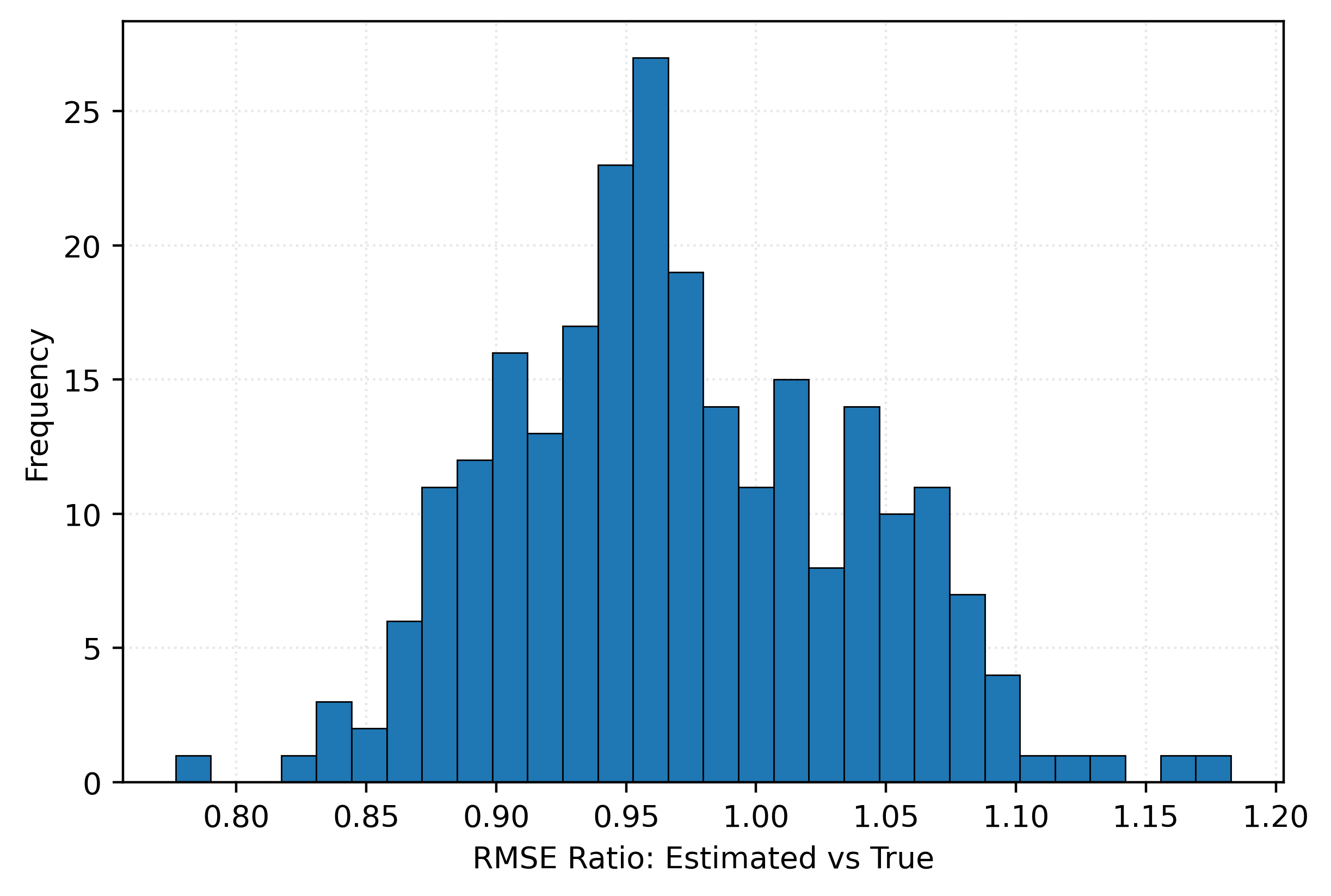

Figure 2: A histogram of the ratios of the estimated versus true RMSE values calculated via a simulation study that incorrectly uses a test set for both selection and evaluation.

Cross-Validation

Now that we understand the need for both a validation and test set, we will further complicate the supervised learning process by introducing cross-validation. We’ll first introduce cross-validation, then explain the issue that it solves.

Let’s show an example of calculating 5-fold cross-validated RMSE for a K-Nearest Neighbors regression model with \(k=3\).

Beware! Unfortunately, there are a limited number of letters in the alphabet. Due to this limitation, some letters are often reused. The “k” in k-fold cross-validation is not the same “k” as the \(k\) in \(k\)-nearest neighbors, which is not the same as the “k” in the \(k\)-means clustering algorithm that we will discuss later.

What is 5-fold cross-validation? 5-fold cross-validation is a specific case of \(k\)-fold cross-validation, where \(k=5\). Essentially, we will split the data into 5 equal parts called “folds.” Each fold will be used as a validation set while the remaining folds are used as the training set, essentially repeating our previous validation process five times. Each time through, we will calculate a metric, for example RMSE. The final cross-validated RMSE will be the average of the five RMSE values.

Figure 3: The Cross-Validation process: data is first split into train and test sets. Then the training data is further divided for 5-fold cross-validation. Each fold takes a turn serving as validation set, while the reamaining folds are used as the train set. Source: Learning Data Science

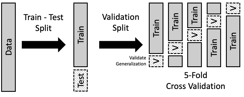
First, we’ll get some data and train-test split it. Then we’ll perform 5-fold cross-validation on the training data.

X, y = simulate_sin_data(
    n=20,
    sd=0.25,
    seed=sim,
)

X_train, X_test, y_train, y_test = train_test_split(
    X,
    y,
    test_size=0.20,
    random_state=42,
)

kf = KFold(n_splits=5, shuffle=True, random_state=42)
knn = KNeighborsRegressor(n_neighbors=3)

rmse_folds = []

for i, (vtrain_idx, validation_idx) in enumerate(kf.split(X_train)):
    print(f" Validation Set: Fold {i + 1}")
    print(f"     Train Indices: {vtrain_idx}")
    print(f"     Validation Indices: {validation_idx}")
    knn.fit(X_train[vtrain_idx, :], y_train[vtrain_idx])
    y_pred = knn.predict(X_train[validation_idx, :])
    rmse_fold = root_mean_squared_error(y_train[validation_idx], y_pred)
    print(f"     Validation RMSE: {rmse_fold:.3f}")
    print(f"")
    rmse_folds.append(rmse_fold)

 Validation Set: Fold 1
     Train Indices: [ 2  3  4  6  7  8  9 10 11 12 13 15]
     Validation Indices: [ 0  1  5 14]
     Validation RMSE: 0.708

 Validation Set: Fold 2
     Train Indices: [ 0  1  2  3  4  5  6  7  9 10 12 14 15]
     Validation Indices: [ 8 11 13]
     Validation RMSE: 0.448

 Validation Set: Fold 3
     Train Indices: [ 0  1  3  4  5  6  7  8 10 11 12 13 14]
     Validation Indices: [ 2  9 15]
     Validation RMSE: 0.403

 Validation Set: Fold 4
     Train Indices: [ 0  1  2  3  5  6  8  9 11 12 13 14 15]
     Validation Indices: [ 4  7 10]
     Validation RMSE: 0.863

 Validation Set: Fold 5
     Train Indices: [ 0  1  2  4  5  7  8  9 10 11 13 14 15]
     Validation Indices: [ 3  6 12]
     Validation RMSE: 0.249

print(f"5-Fold Cross-Validated RMSE: {np.mean(rmse_folds):.3f}")

5-Fold Cross-Validated RMSE: 0.534

Why would we need to do this? Doesn’t this just make things more complicated? Doesn’t this just waste a bunch of time? We’re just repeating the same thing five times!

Let’s perform another simulation study. This time we’ll compare the results of selecting a model with a single validation set versus selecting a model with 5-fold cross-validation.

# here we define the values of k we will consider
k_values = np.arange(1, 11)

Tuning with Single Validation Set

# store the best k value for each simulation
k_best = []

# run 100 different simulations to assess k selection stability
for seed in range(100):

    # generate a new dataset for this simulation
    X, y = simulate_sin_data(n=50, sd=0.25, seed=sim)

    # split into training and test sets
    X_train, X_test, y_train, y_test = train_test_split(
        X,
        y,
        test_size=0.20,
        random_state=seed,
    )

    # further split training data into train/validation for hyperparameter tuning
    X_vtrain, X_validation, y_vtrain, y_validation = train_test_split(
        X_train,
        y_train,
        test_size=0.20,
        random_state=seed,
    )

    # store RMSE for each k value
    k_rmse = []

    # test each k value using validation set
    for k in k_values:
        knn = KNeighborsRegressor(n_neighbors=k)
        knn.fit(X_vtrain, y_vtrain)
        k_rmse.append(root_mean_squared_error(y_validation, knn.predict(X_validation)))

    # find and store the k value with lowest validation error
    k_best.append(k_values[np.argmin(k_rmse)])

np.array(k_best)

array([ 6,  6,  6,  2,  5,  2,  6,  2,  9,  4,  1,  2,  6,  7,  2,  3,  3,
        1,  1,  3,  1,  2,  3,  3,  2,  3,  2,  1,  2,  3,  5,  2,  2,  1,
        5,  4,  5,  2,  4,  2,  2,  5,  2, 10,  5,  1,  7,  3,  3,  4,  3,
        2,  6,  1,  6,  1,  2,  4,  4,  1,  1,  4,  4,  6,  2,  4,  2,  4,
        4,  3,  3,  3,  3,  4,  1,  3,  5,  2,  4,  2,  3,  3,  2,  6,  3,
        1,  5,  4,  3,  4,  4,  3,  2,  5,  1,  1,  3,  3,  1,  3])

fig, ax = plt.subplots()
ax.bar(k_values, [k_best.count(i) for i in k_values])
ax.set_title("Repeatedly Tuning k: Single Validation Set")
ax.set_xlabel("k")
ax.set_ylabel("Times Selected")
ax.set_xticks(k_values)
plt.show()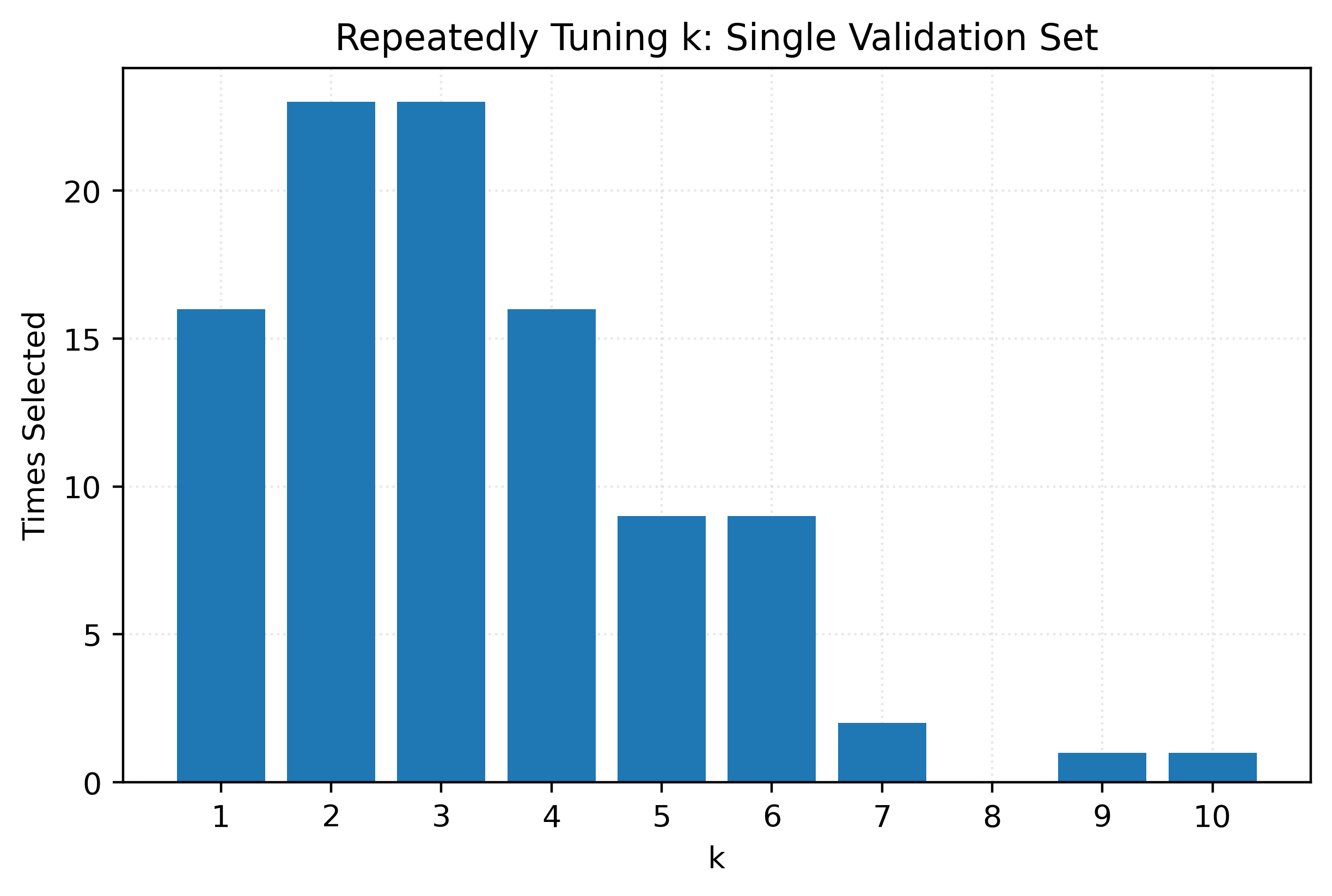

Tuning with Cross-Validation

# store the best k value for each simulation
k_best = []

# run 100 different simulations to assess k selection stability
for seed in range(100):

    # generate a new dataset for this simulation
    X, y = simulate_sin_data(
        n=50,
        sd=0.25,
        seed=sim,
    )

    # split into training and test sets
    X_train, X_test, y_train, y_test = train_test_split(
        X,
        y,
        test_size=0.20,
        random_state=seed,
    )

    # store RMSE for each k value
    k_rmse = []

    # test each k value using cross-validation
    for k in k_values:
        knn = KNeighborsRegressor(n_neighbors=k)
        # perform 5-fold cross-validation on training data
        cv_scores = cross_val_score(
            knn,
            X_train,
            y_train,
            cv=5,
            scoring="neg_root_mean_squared_error",
        )
        # convert negative RMSE back to positive and store mean
        k_rmse.append(-np.mean(cv_scores))

    # find and store the k value with lowest CV error
    k_best.append(k_values[np.argmin(k_rmse)])

np.array(k_best)

array([4, 1, 4, 6, 3, 3, 5, 4, 2, 3, 4, 2, 4, 4, 4, 2, 3, 4, 2, 3, 2, 2,
       2, 3, 3, 3, 4, 1, 4, 2, 4, 4, 3, 1, 4, 3, 2, 3, 4, 4, 4, 3, 5, 4,
       3, 4, 4, 1, 3, 2, 3, 2, 5, 3, 4, 3, 4, 3, 4, 2, 1, 2, 3, 4, 3, 4,
       3, 3, 3, 3, 3, 3, 4, 6, 2, 2, 3, 3, 3, 1, 3, 3, 3, 3, 2, 5, 2, 4,
       4, 3, 4, 4, 2, 2, 1, 3, 4, 3, 1, 2])

fig, ax = plt.subplots()
ax.bar(k_values, [k_best.count(i) for i in k_values])
ax.set_title("Repeatedly Tuning k: 5-Fold Cross-Validation")
ax.set_xlabel("k")
ax.set_ylabel("Times Selected")
ax.set_xticks(k_values)
plt.show()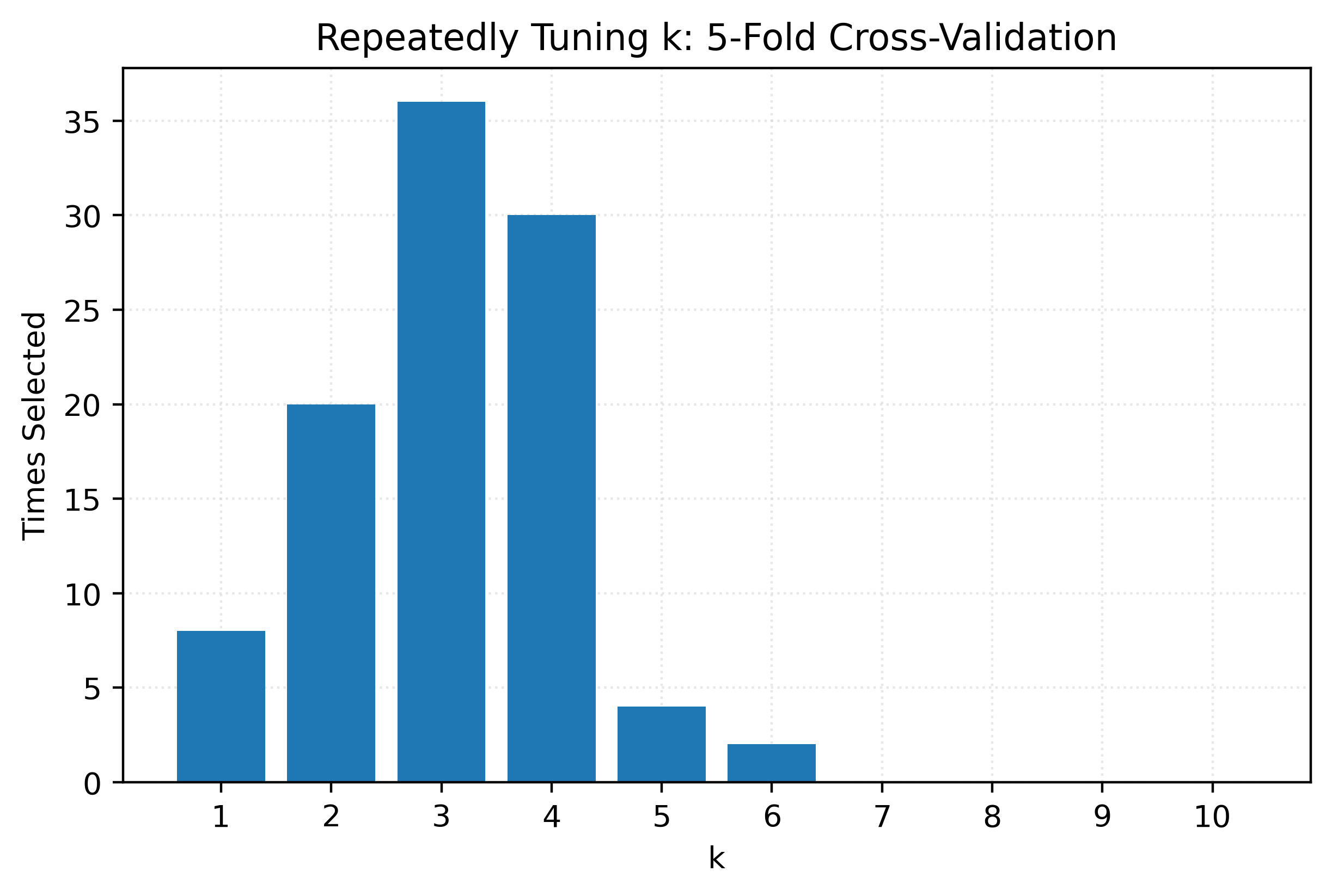

Grid Search

So far, we’ve demonstrated two things:

• The need for both validation and test data.
• The need for cross-validation.

But while we’ve shown that we need to do these things, we haven’t shown how to do them efficiently. The code we’ve written so far is not the code you would write in practice.

Instead, in practice you will want to use the GridSearchCV class, together with a Pipeline. Combining these two tools will demonstrate the true power of sklearn. At times you might need something more custom, or an alternative to GridSearchCV, but for most cases, GridSearchCV and a Pipeline will be your go-to when using sklearn to perform supervised learning.

By using GridSearchCV and a Pipeline, rather than writing for loops and other verbose code to perform parameter tuning, instead you can focus on specifying the inputs to the process. As the human in the loop, you will need to specify:

• The model(s) you want to tune.
• The hyperparameters you want to tune.
• The values you want to consider for each hyperparameter.
• The metric you want to use to evaluate the models.
• The number of folds for cross-validation.
• The preprocessing steps you want to include in the pipeline.

Let’s take a look at an example.

Example: Palmer Penguins

penguins = load_penguins()

penguins_train, penguins_test = train_test_split(
    penguins,
    test_size=0.35,
    random_state=42,
)

penguins_train

	species	island	bill_length_mm	bill_depth_mm	flipper_length_mm	body_mass_g	sex	year
292	Chinstrap	Dream	50.30	20.00	197.00	3,300.00	male	2007
302	Chinstrap	Dream	50.50	18.40	200.00	3,400.00	female	2008
56	Adelie	Biscoe	39.00	17.50	186.00	3,550.00	female	2008
271	Gentoo	Biscoe	NaN	NaN	NaN	NaN	NaN	2009
10	Adelie	Torgersen	37.80	17.10	186.00	3,300.00	NaN	2007
...	...	...	...	...	...	...	...	...
188	Gentoo	Biscoe	42.60	13.70	213.00	4,950.00	female	2008
71	Adelie	Torgersen	39.70	18.40	190.00	3,900.00	male	2008
106	Adelie	Biscoe	38.60	17.20	199.00	3,750.00	female	2009
270	Gentoo	Biscoe	47.20	13.70	214.00	4,925.00	female	2009
102	Adelie	Biscoe	37.70	16.00	183.00	3,075.00	female	2009

223 rows × 8 columns

plot = sns.jointplot(
    data=penguins_train,
    x="bill_length_mm",
    y="bill_depth_mm",
    hue="species",
    edgecolor="k",
    alpha=0.75,
    space=0,
)
plot.set_axis_labels(
    xlabel="Bill Length (mm)",
    ylabel="Bill Depth (mm)",
)
plot.ax_joint.legend(
    title="Species",
    loc="lower left",
)
plt.show()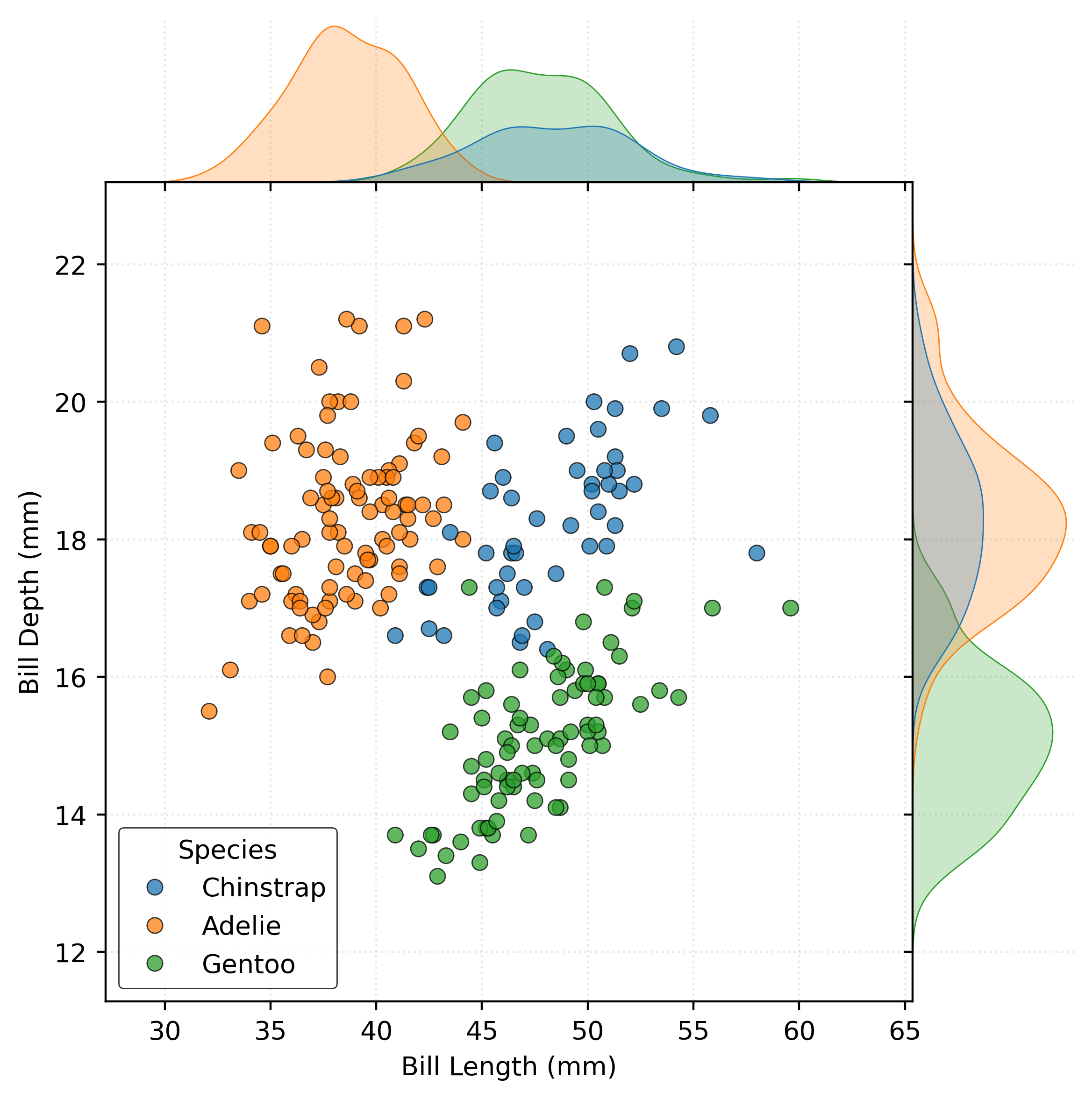

numeric_features = ["bill_length_mm", "bill_depth_mm", "body_mass_g"]
categorical_features = ["sex"]
features = numeric_features + categorical_features
target = "species"

X_train = penguins_train[features]
y_train = penguins_train[target]

X_test = penguins_test[features]
y_test = penguins_test[target]

# define preprocessing for numeric features
numeric_transformer = Pipeline(
    [
        ("imputer", SimpleImputer(strategy="median")),
        ("scaler", StandardScaler()),
    ]
)

# define preprocessing for categorical features
categorical_transformer = Pipeline(
    [
        ("imputer", SimpleImputer(strategy="most_frequent")),
        ("encoder", OneHotEncoder()),
    ]
)

# create general preprocessor
preprocessor = ColumnTransformer(
    [
        ("numeric", numeric_transformer, numeric_features),
        ("categorical", categorical_transformer, categorical_features),
    ],
    remainder="drop",
)

# create pipeline with preprocessor and classifier
pipeline = Pipeline(
    [
        ("preprocessor", preprocessor),
        ("classifier", KNeighborsClassifier()),
    ]
)

# define the parameter grid
param_grid = {
    "classifier__n_neighbors": [1, 5, 10, 15, 20, 25, 50],
    "classifier__p": [1, 2],
    "preprocessor__numeric__scaler": [None, StandardScaler()],
}

# create the grid search
mod = GridSearchCV(
    pipeline,
    param_grid,
    cv=5,
    scoring="accuracy",
)

mod

GridSearchCV(cv=5,
             estimator=Pipeline(steps=[('preprocessor',
                                        ColumnTransformer(transformers=[('numeric',
                                                                         Pipeline(steps=[('imputer',
                                                                                          SimpleImputer(strategy='median')),
                                                                                         ('scaler',
                                                                                          StandardScaler())]),
                                                                         ['bill_length_mm',
                                                                          'bill_depth_mm',
                                                                          'body_mass_g']),
                                                                        ('categorical',
                                                                         Pipeline(steps=[('imputer',
                                                                                          SimpleImputer(strategy='most_frequent')),
                                                                                         ('encoder',
                                                                                          OneHotEncoder())]),
                                                                         ['sex'])])),
                                       ('classifier', KNeighborsClassifier())]),
             param_grid={'classifier__n_neighbors': [1, 5, 10, 15, 20, 25, 50],
                         'classifier__p': [1, 2],
                         'preprocessor__numeric__scaler': [None,
                                                           StandardScaler()]},
             scoring='accuracy')

In a Jupyter environment, please rerun this cell to show the HTML representation or trust the notebook.
On GitHub, the HTML representation is unable to render, please try loading this page with nbviewer.org.

# fit the model via grid search
mod.fit(X_train, y_train)

GridSearchCV(cv=5,
             estimator=Pipeline(steps=[('preprocessor',
                                        ColumnTransformer(transformers=[('numeric',
                                                                         Pipeline(steps=[('imputer',
                                                                                          SimpleImputer(strategy='median')),
                                                                                         ('scaler',
                                                                                          StandardScaler())]),
                                                                         ['bill_length_mm',
                                                                          'bill_depth_mm',
                                                                          'body_mass_g']),
                                                                        ('categorical',
                                                                         Pipeline(steps=[('imputer',
                                                                                          SimpleImputer(strategy='most_frequent')),
                                                                                         ('encoder',
                                                                                          OneHotEncoder())]),
                                                                         ['sex'])])),
                                       ('classifier', KNeighborsClassifier())]),
             param_grid={'classifier__n_neighbors': [1, 5, 10, 15, 20, 25, 50],
                         'classifier__p': [1, 2],
                         'preprocessor__numeric__scaler': [None,
                                                           StandardScaler()]},
             scoring='accuracy')

In a Jupyter environment, please rerun this cell to show the HTML representation or trust the notebook.
On GitHub, the HTML representation is unable to render, please try loading this page with nbviewer.org.

print(f"Best Parameters:")
pprint(mod.best_params_)

Best Parameters:
{'classifier__n_neighbors': 1,
 'classifier__p': 1,
 'preprocessor__numeric__scaler': StandardScaler()}

print(f"Best Cross-Validated Accuracy: {mod.best_score_}")

Best Cross-Validated Accuracy: 0.9821212121212122

# create a DataFrame to store the CV results
cv_results = pd.DataFrame(mod.cv_results_)

# select relevant columns and sort by rank
cv_results = (
    cv_results[
        [
            "param_classifier__n_neighbors",
            "param_classifier__p",
            "param_preprocessor__numeric__scaler",
            "mean_test_score",
            "std_test_score",
        ]
    ]
    .sort_values(by="mean_test_score", ascending=False)
    .reset_index(drop=True)
)

# rename columns for better readability
cv_results.columns = [
    "Neighbors",
    "Distance Exponent",
    "Scaling",
    "Mean Accuracy",
    "SD Accuracy",
]

# display the DataFrame
cv_results

	Neighbors	Distance Exponent	Scaling	Mean Accuracy	SD Accuracy
0	1	1	StandardScaler()	0.9821	0.0167
1	10	2	StandardScaler()	0.9820	0.0170
2	5	1	StandardScaler()	0.9776	0.0283
3	1	2	StandardScaler()	0.9776	0.0201
4	5	2	StandardScaler()	0.9776	0.0201
5	15	2	StandardScaler()	0.9775	0.0249
6	25	2	StandardScaler()	0.9730	0.0168
7	20	2	StandardScaler()	0.9729	0.0223
8	15	1	StandardScaler()	0.9685	0.0231
9	10	1	StandardScaler()	0.9685	0.0231
10	20	1	StandardScaler()	0.9596	0.0170
11	25	1	StandardScaler()	0.9418	0.0301
12	50	2	StandardScaler()	0.9279	0.0441
13	1	2	None	0.8433	0.0415
14	1	1	None	0.8343	0.0404
15	50	1	StandardScaler()	0.8341	0.0171
16	5	1	None	0.7799	0.0406
17	5	2	None	0.7799	0.0406
18	15	1	None	0.7755	0.0396
19	15	2	None	0.7755	0.0396
20	10	2	None	0.7664	0.0661
21	10	1	None	0.7664	0.0661
22	25	2	None	0.7400	0.0163
23	20	2	None	0.7398	0.0373
24	25	1	None	0.7355	0.0160
25	20	1	None	0.7354	0.0415
26	50	1	None	0.7220	0.0171
27	50	2	None	0.7220	0.0171

# predict on the test data
y_test_pred = mod.predict(X_test)

# calculate and print the test accuracy
test_accuracy = accuracy_score(y_test, y_test_pred)
print(f"Test Accuracy: {test_accuracy}")

Test Accuracy: 0.9834710743801653

TODO

• Why CV? Why not just a single validation set?

  • Variability in selection!
  • Also estimate of uncertainty as opposite to just an estimate of performance

• With GridSearchCV, also show “full” pipeline details, including naming steps?

  • Do this as a part of “reviewing” supervised learning leading into exam instead.

• Note that this note is very tied to generalization, but will be presented more mechanically and justified separately.

• https://scikit-learn.org/stable/modules/generated/sklearn.model_selection.cross_val_score.html

  • https://scikit-learn.org/stable/modules/cross_validation.html#cross-validation

• https://scikit-learn.org/stable/modules/generated/sklearn.model_selection.GridSearchCV.html

  • https://scikit-learn.org/stable/modules/mod.html#grid-search

• https://scikit-learn.org/stable/modules/generated/sklearn.model_selection.KFold.html

  • https://scikit-learn.org/stable/modules/cross_validation.html#k-fold

• scoring names: https://scikit-learn.org/stable/modules/model_evaluation.html#string-name-scorers

• https://scikit-learn.org/stable/modules/model_evaluation.html