# basics
import numpy as np
import matplotlib.pyplot as plt
import pandas as pd
import seaborn as sns

# machine learning
from sklearn.datasets import make_friedman1, make_regression
from sklearn.tree import DecisionTreeRegressor, plot_tree, export_text
from sklearn.neighbors import KNeighborsRegressor
from sklearn.metrics import root_mean_squared_error, mean_squared_error, r2_score
from sklearn.model_selection import train_test_split

# data
from ucimlrepo import fetch_ucirepoDecision Trees for Regression
Neighborhoods via Recursive Partitioning
Objectives
In this note, we will discuss:
- decision trees for regression,
- how trees differ from KNN when determining similarity of data,
- how to find and evaluate decision tree splits for regression,
- and how to fit and tune decision trees with
DecisionTreeRegressor.
We’ll return to the Auto MPG example to explore how trees split data and make predictions.
Python Setup
Notebook
The following Jupyter notebook contains some starter code that may be useful for following along with this note.
Introduction
Decision trees are a fundamental machine learning algorithm that can be used for both classification and regression tasks. In regression problems, decision trees predict numeric target variables by recursively partitioning the feature space into regions (“neighborhoods”) and predicting the mean (or other statistics like the median) of the target values within each region.
Loss Functions
\[ \text{MSE}(y, \hat{y}) = \frac{1}{n}\sum_{i=1}^{n} (y_i - \hat{y})^2 \]
\[ \text{MAE}(y, \hat{y}) = \frac{1}{n}\sum_{i=1}^{n} \left| (y_i - \hat{y}) \right| \]
\[ \text{SSE}(y, \hat{y}) = \sum_{i=1}^{n} (y_i - \hat{y})^2 \]
Tree Building Idea
| \(x\) | \(y\) |
|---|---|
| 2.65 | 2.52 |
| 7.96 | 7.05 |
| 6.12 | 6.35 |
| 9.18 | 6.82 |
| 3.47 | 3.08 |
| 9.80 | 7.09 |
| 5.31 | 6.21 |
| 5.10 | 6.53 |
| 6.53 | 6.50 |
| 3.88 | 2.65 |
Decision trees split the feature data into regions (neighborhoods), called nodes, by finding optimal cutoffs.
For a single feature \(x\) and node \(N\), we choose a cutoff value \(c_N\) that divides our data into two groups:
- Left Node: \(N_L = \{i : x_i \leq c_N\}\)
- Right Node: \(N_R = \{i : x_i > c_N\}\)
Each neighborhood predicts the mean of the target values within that region.
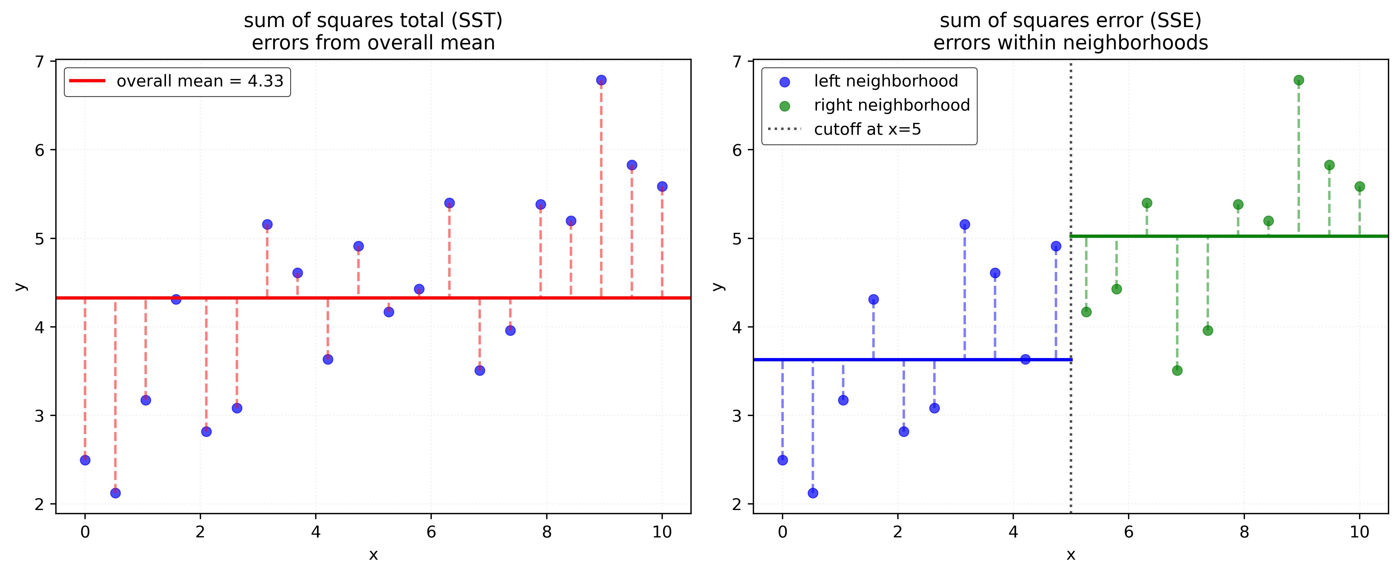
To find the optimal split, we consider all possible features (here just a single feature \(x\)) and all possible cutoff values, then choose the combination that minimizes \(\text{SSE}\).
After splitting node \(N\) based on \(x_j \leq c_N\), the new \(\text{SSE}\) is:
\[ \text{SSE}(y, \hat{y}) = \sum_{i=1}^{n} (y_i - \hat{y})^2 = \sum_{i \in N_L} (y_i - \bar{y}_L)^2 + \sum_{i \in N_R} (y_i - \bar{y}_R)^2 \]
where \(\bar{y}_L\) and \(\bar{y}_R\) are the means of the left and right nodes, respectively. That is, for samples in the left node, \(N_L\), the predicted value \(\hat{y}\) is \(\bar{y}_L\). For samples in the right node, \(N_R\), the predicted value \(\hat{y}\) is \(\bar{y}_R\).
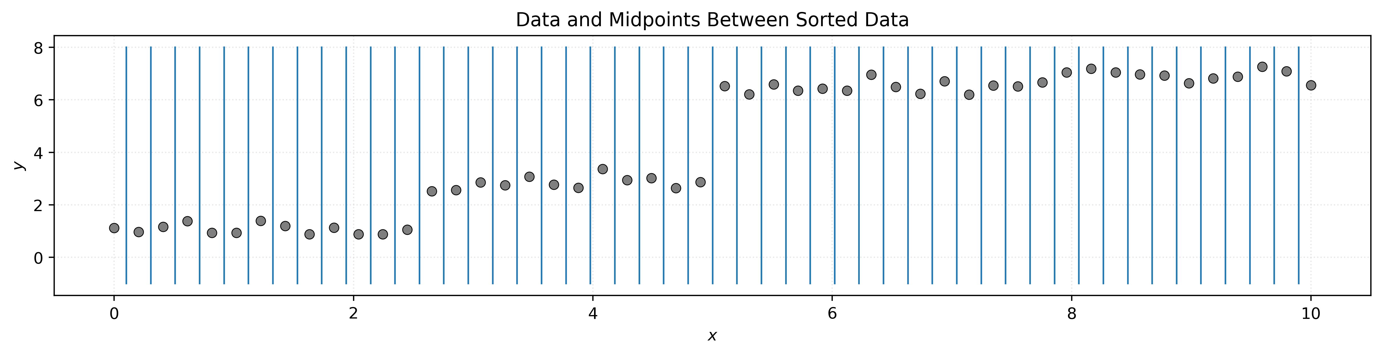
The algorithm considers all features and typically uses midpoints between adjacent sorted values as potential cutoffs.
A tree will consist of more than a single split. To develop a “deeper” tree, we recursively partition the feature space. That is, after splitting the root node \(N_0\) into nodes \(N_L\) and \(N_R\), we repeat the same process within both nodes.
We first split \(N_L\) into \(N_{LL}\) and \(N_{LR}\).
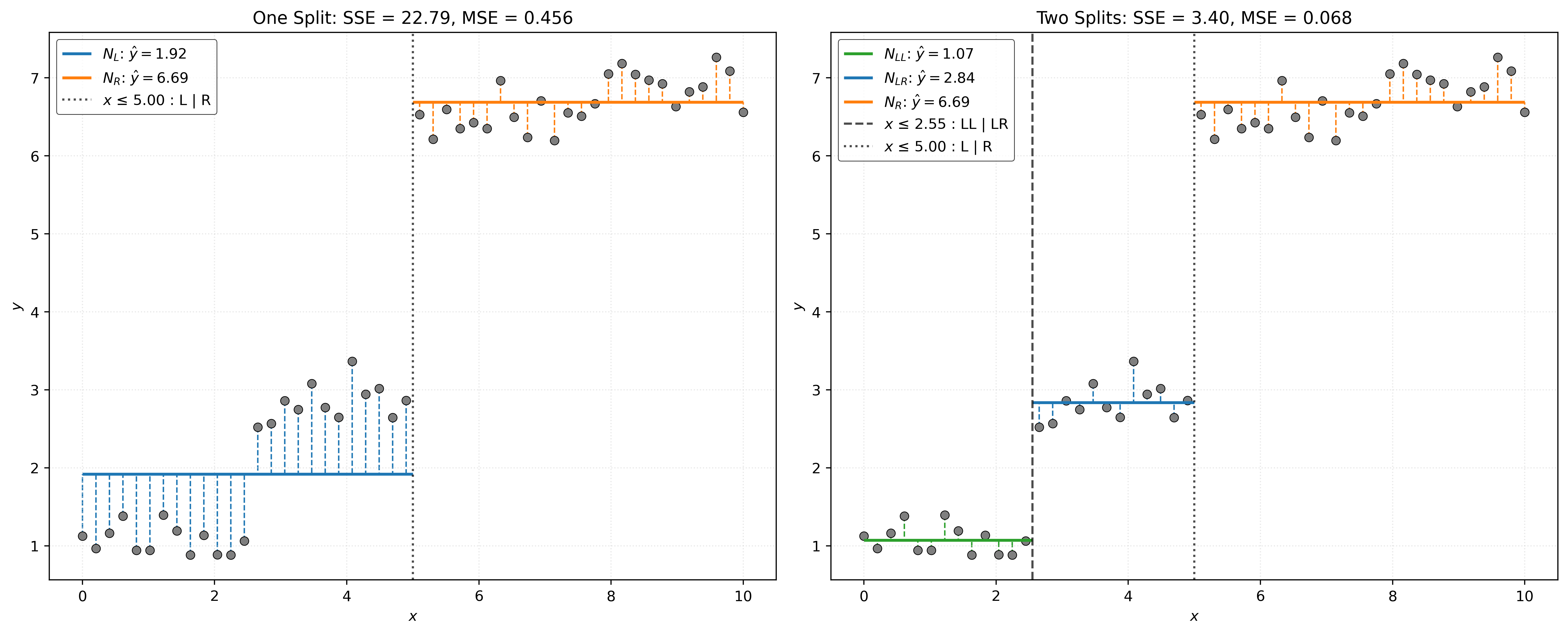
With an arbitrary number of neighborhoods \(T\) (terminal nodes), we have:
\[ \text{SSE}(y, \hat{y}) = \sum_{t=1}^{T} \sum_{i \in N_t} (y_i - \bar{y}_t)^2 \]
We then split \(N_R\) into \(N_{RL}\) and \(N_{RR}\).
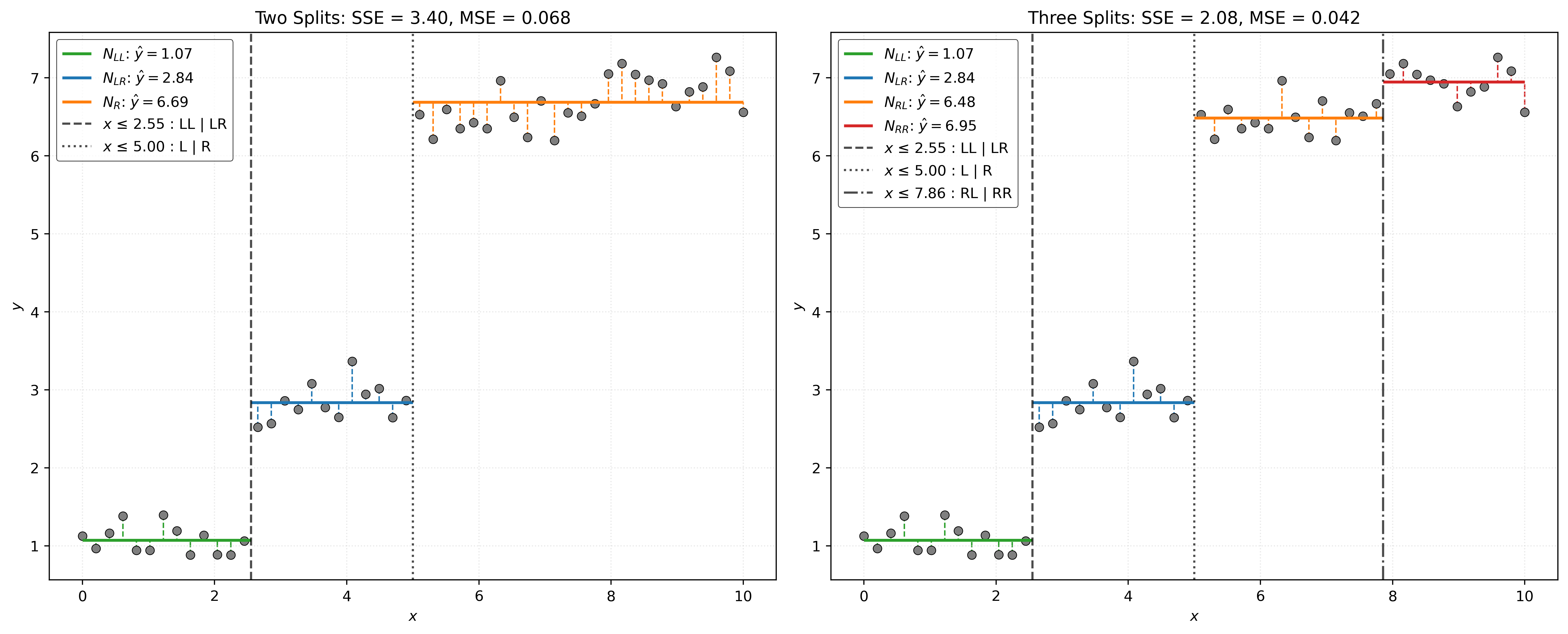
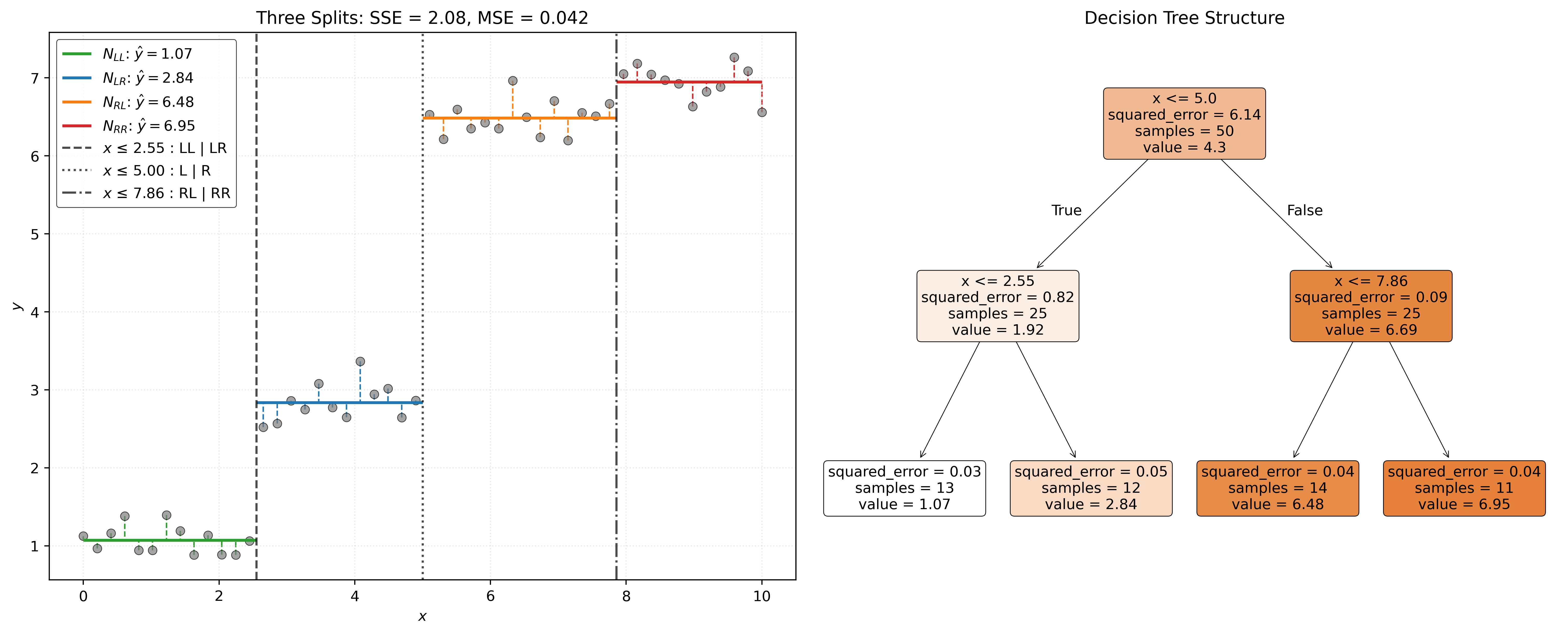
With a tree build, we can give categorize the different types of nodes that we have encountered.
- Root Node: The “top” node containing all data.
- Terminal Nodes: Nodes at the “bottom” of the tree that are not split any further. In the tree analogy, this could also be called leaves.
- Internal Nodes: Any node that is not the root node or a terminal node.
Decision Tree Tuning Parameters
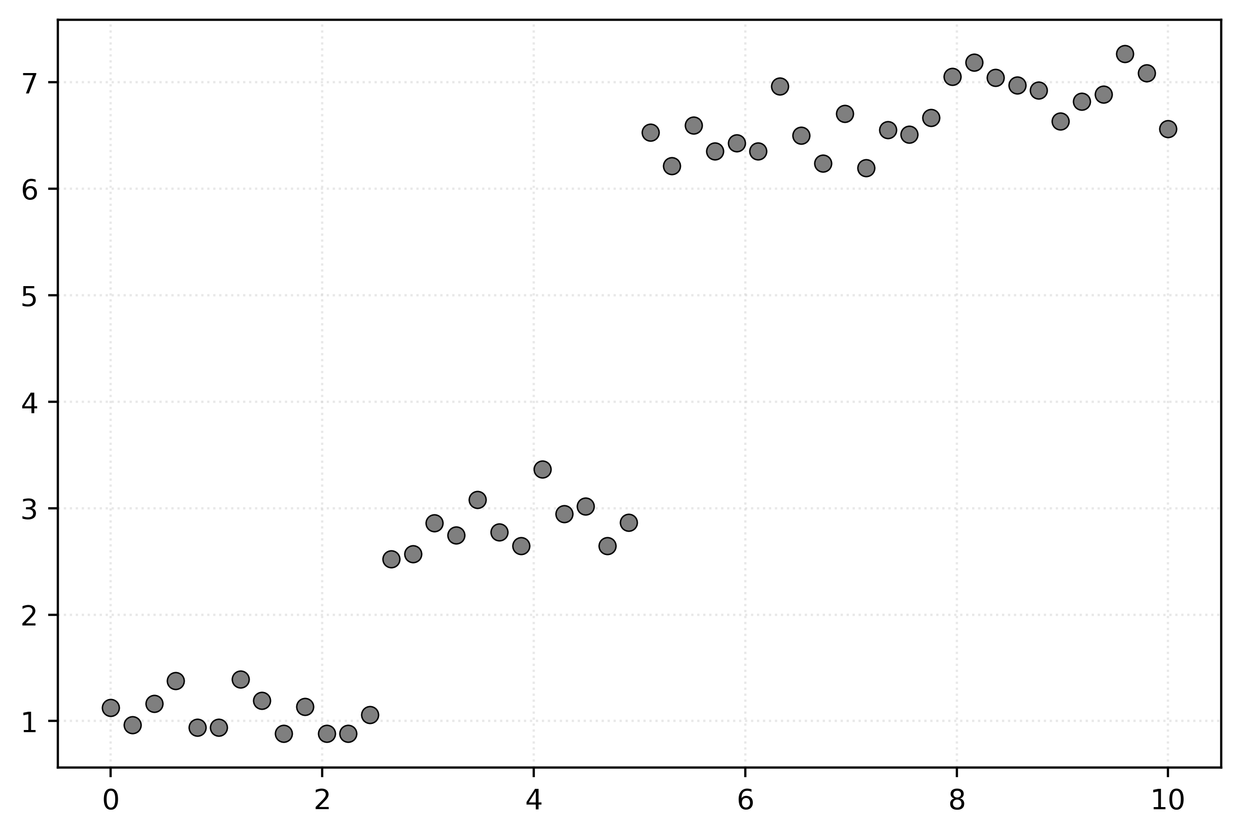
def simulate_sin_data(n, sd, seed):
    np.random.seed(seed)
    X = np.random.uniform(
        low=-2 * np.pi,
        high=2 * np.pi,
        size=(n, 1),
    )
    signal = np.sin(X).ravel()
    noise = np.random.normal(
        loc=0,
        scale=sd,
        size=n,
    )
    y = signal + noise
    return X, y
X, y = simulate_sin_data(n=200, sd=0.25, seed=42)Show Code for Plot
# setup figure
fig, axs = plt.subplots(1, 2, figsize=(12, 5))

# x values to make predictions at for plotting purposes
x_plot = np.linspace(-2 * np.pi, 2 * np.pi, 1000).reshape((1000, 1))

# create subplot for "simulation study"
axs[0].set_title("Simulation Study")
axs[0].scatter(X, y, s=50, alpha=0.5, c="tab:gray")
axs[0].plot(x_plot, np.sin(x_plot), zorder=3)
axs[0].set_xlabel("$x$")
axs[0].set_ylabel("$y$")

# create subplot for "reality"
axs[1].set_title("Reality")
axs[1].scatter(X, y, s=50, alpha=0.5, c="tab:gray")
axs[1].set_xlabel("$x$")

# show plot
plt.show()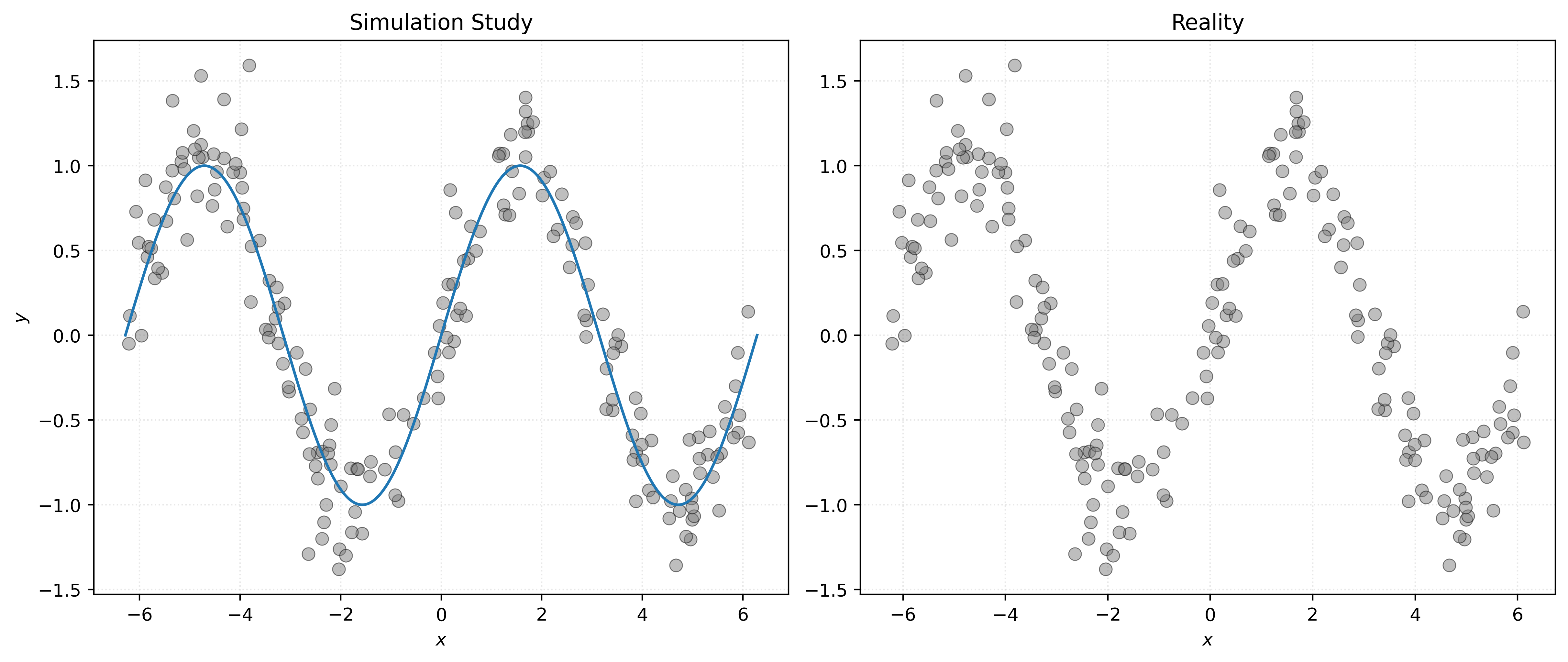
# fit a knn model for comparison
knn010 = KNeighborsRegressor(n_neighbors=10)
_ = knn010.fit(X, y)
# list the possible parameters (and their default values) to the DecisionTreeRegressor
DecisionTreeRegressor().get_params(){'ccp_alpha': 0.0,
'criterion': 'squared_error',
'max_depth': None,
'max_features': None,
'max_leaf_nodes': None,
'min_impurity_decrease': 0.0,
'min_samples_leaf': 1,
'min_samples_split': 2,
'min_weight_fraction_leaf': 0.0,
'monotonic_cst': None,
'random_state': None,
'splitter': 'best'}# fit a decision tree with min_samples_split=40
dt040 = DecisionTreeRegressor(min_samples_split=40)
_ = dt040.fit(X, y)Show Code for Plot
# setup figure
fig, axs = plt.subplots(1, 2, figsize=(12, 5))

# create subplot for KNN
axs[0].set_title("k-Nearest Neighbors, $k=10$")
axs[0].scatter(X, y, s=50, alpha=0.5, c="tab:gray")
axs[0].plot(x_plot, knn010.predict(x_plot))
axs[0].set_xlabel("$x$")
axs[0].set_ylabel("$y$")

# create subplot for decision tree
axs[1].set_title(r"Decision Tree, $\mathtt{min\_samples\_split=40}$")
axs[1].scatter(X, y, s=50, alpha=0.5, c="tab:gray")
axs[1].plot(x_plot, dt040.predict(x_plot))
axs[0].set_xlabel("$x$")

# show plot
plt.show()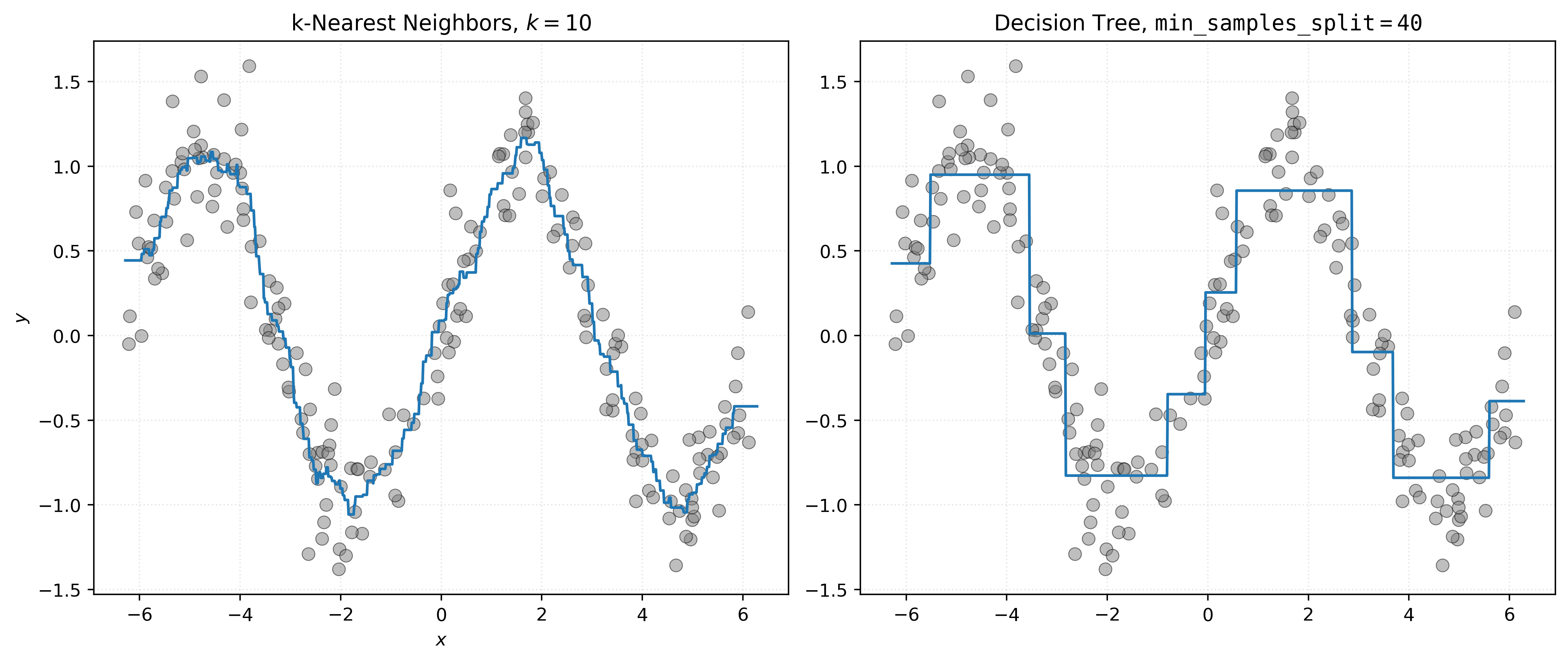
# visualize the decision tree
fig, ax = plt.subplots(1, 1, figsize=(12, 8))
plot_tree(dt040, feature_names=["x"], filled=True, rounded=True, fontsize=10, precision=2)
plt.show()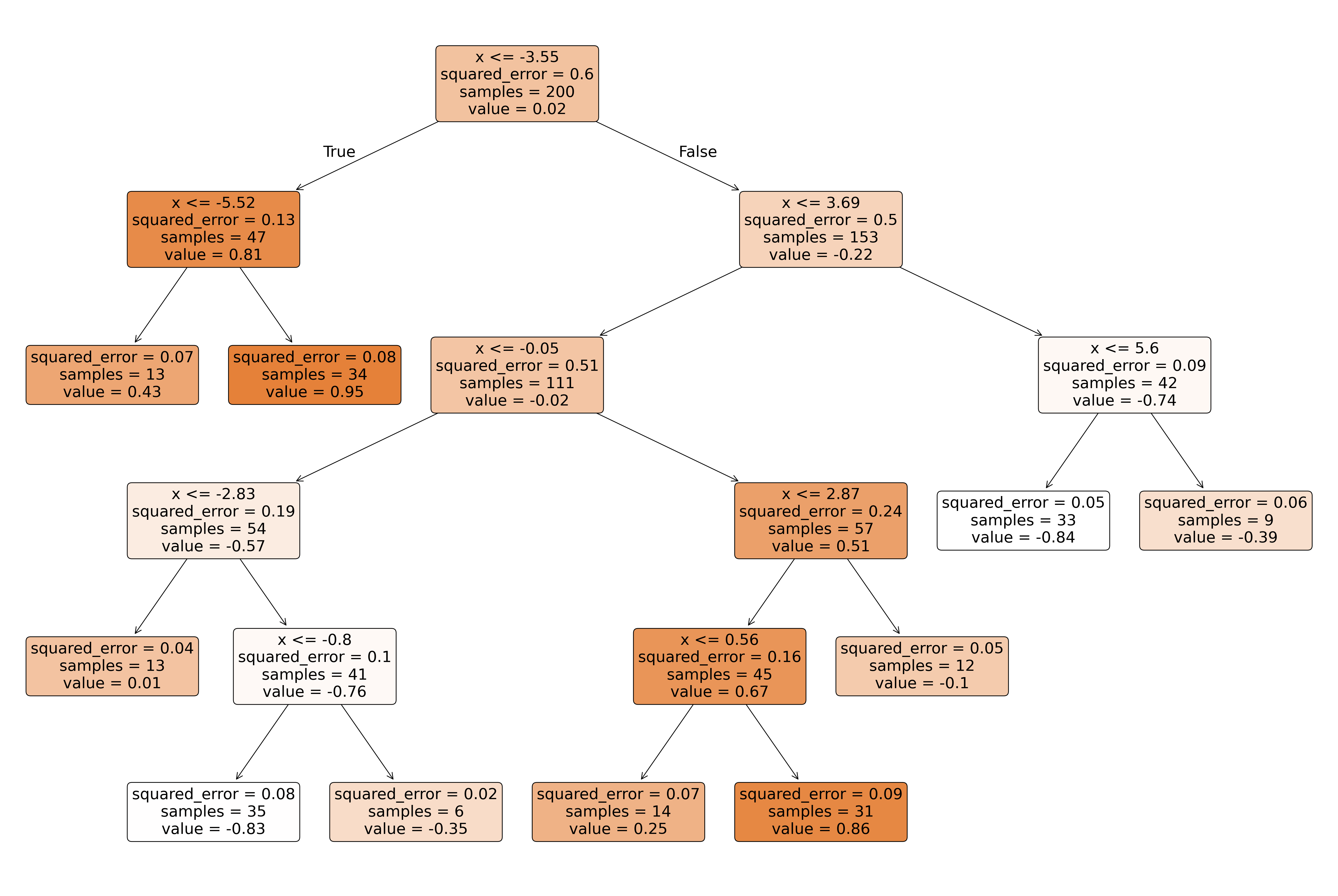
# view text representation of the tree
print(export_text(dt040))
|--- feature_0 <= -3.55
| |--- feature_0 <= -5.52
| | |--- value: [0.43]
| |--- feature_0 > -5.52
| | |--- value: [0.95]
|--- feature_0 > -3.55
| |--- feature_0 <= 3.69
| | |--- feature_0 <= -0.05
| | | |--- feature_0 <= -2.83
| | | | |--- value: [0.01]
| | | |--- feature_0 > -2.83
| | | | |--- feature_0 <= -0.80
| | | | | |--- value: [-0.83]
| | | | |--- feature_0 > -0.80
| | | | | |--- value: [-0.35]
| | |--- feature_0 > -0.05
| | | |--- feature_0 <= 2.87
| | | | |--- feature_0 <= 0.56
| | | | | |--- value: [0.25]
| | | | |--- feature_0 > 0.56
| | | | | |--- value: [0.86]
| | | |--- feature_0 > 2.87
| | | | |--- value: [-0.10]
| |--- feature_0 > 3.69
| | |--- feature_0 <= 5.60
| | | |--- value: [-0.84]
| | |--- feature_0 > 5.60
| | | |--- value: [-0.39]
# initialize decision trees with different values of the tuning parameter min_samples_split
dt002 = DecisionTreeRegressor(min_samples_split=2)
dt100 = DecisionTreeRegressor(min_samples_split=100)
dt250 = DecisionTreeRegressor(min_samples_split=250)
# fit those models
_ = dt002.fit(X, y)
_ = dt100.fit(X, y)
_ = dt250.fit(X, y)Show Code for Plot
# setup figure
fig, axs = plt.subplots(1, 3, figsize=(18, 5))

# create subplot for decision tree with min_samples_split=250
axs[0].set_title(r"$\mathtt{min\_samples\_split=250}$")
axs[0].scatter(X, y, s=50, alpha=0.5, c="tab:gray")
axs[0].plot(x_plot, dt250.predict(x_plot))
axs[0].set_xlabel("$x$")
axs[0].set_ylabel("$y$")

# create subplot for decision tree with min_samples_split=100
axs[1].set_title(r"$\mathtt{min\_samples\_split=100}$")
axs[1].scatter(X, y, s=50, alpha=0.5, c="tab:gray")
axs[1].plot(x_plot, dt100.predict(x_plot))
axs[1].set_xlabel("$x$")

# create subplot for decision tree with min_samples_split=2
axs[2].set_title(r"$\mathtt{min\_samples\_split=2}$")
axs[2].scatter(X, y, s=50, alpha=0.5, c="tab:gray")
axs[2].plot(x_plot, dt002.predict(x_plot))
axs[2].set_xlabel("$x$")

# show plot
plt.show()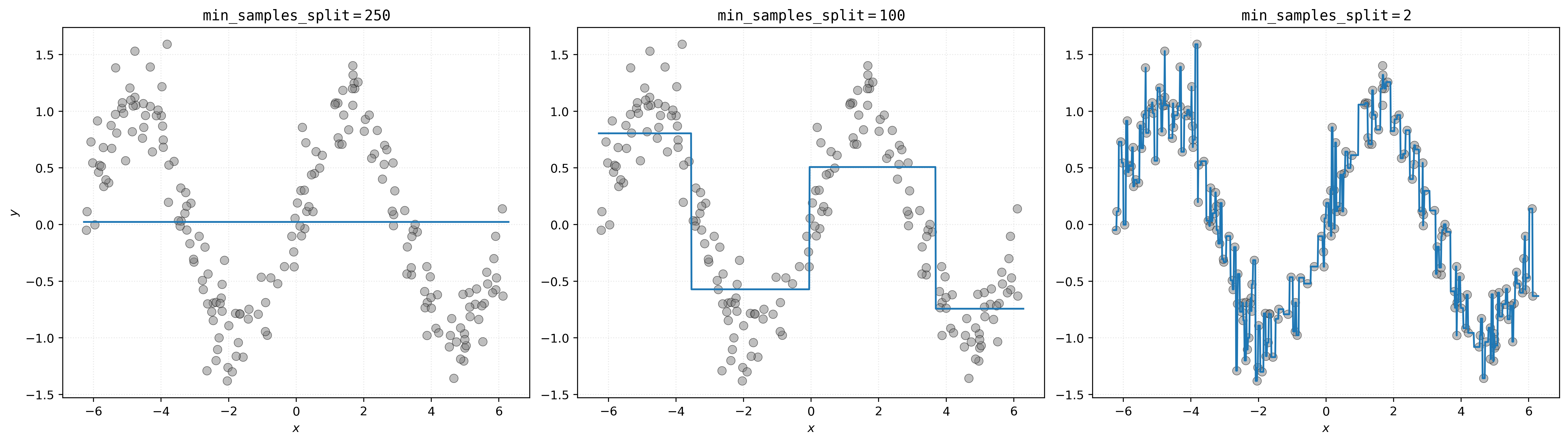
# initialize decision trees with different values of the tuning parameter max_depth
dt_d01 = DecisionTreeRegressor(max_depth=1)
dt_d05 = DecisionTreeRegressor(max_depth=5)
dt_d10 = DecisionTreeRegressor(max_depth=10)
# fit those models
_ = dt_d01.fit(X, y)
_ = dt_d05.fit(X, y)
_ = dt_d10.fit(X, y)Show Code for Plot
# setup figure
fig, axs = plt.subplots(1, 3, figsize=(18, 5))

# create subplot for decision tree with max_depth=1
axs[0].set_title(r"$\mathtt{max\_depth=1}$")
axs[0].scatter(X, y, s=50, alpha=0.5, c="tab:gray")
axs[0].plot(x_plot, dt_d01.predict(x_plot))
axs[0].set_xlabel("$x$")
axs[0].set_ylabel("$y$")

# create subplot for decision tree with max_depth=5
axs[1].set_title(r"$\mathtt{max\_depth=5}$")
axs[1].scatter(X, y, s=50, alpha=0.5, c="tab:gray")
axs[1].plot(x_plot, dt_d05.predict(x_plot))
axs[1].set_xlabel("$x$")

# create subplot for decision tree with max_depth=10
axs[2].set_title(r"$\mathtt{max\_depth=10}$")
axs[2].scatter(X, y, s=50, alpha=0.5, c="tab:gray")
axs[2].plot(x_plot, dt_d10.predict(x_plot))
axs[2].set_xlabel("$x$")

# show plot
plt.show()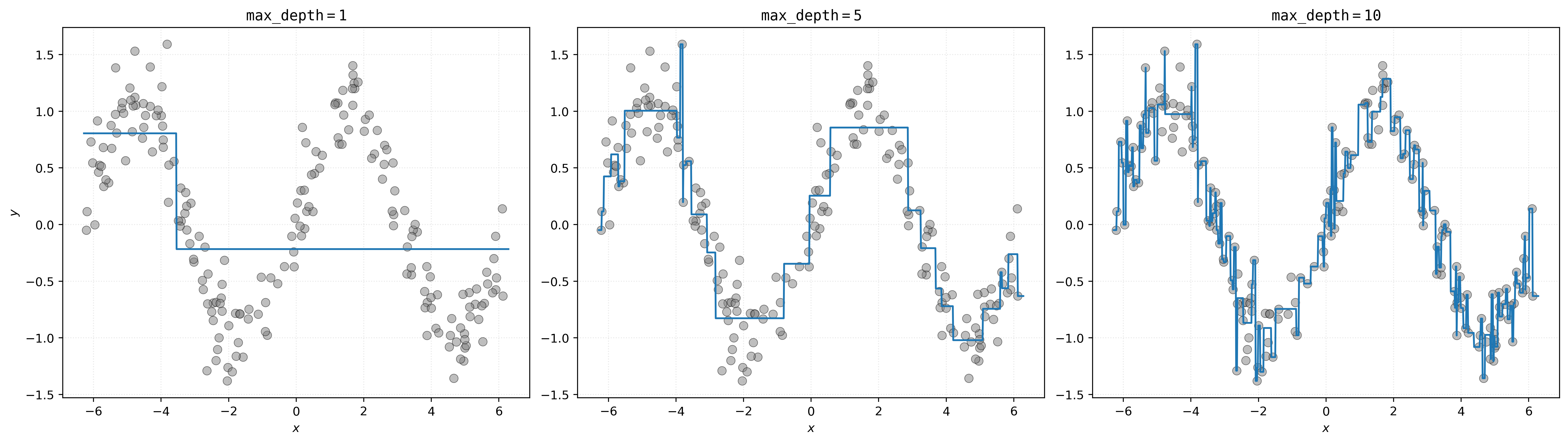
Recursive Partitioning Algorithm
The decision tree algorithm works through recursive partitioning. Let’s look at a sketch of the algorithm.
- Initialize root node containing all data.
- Set stop conditions via
min_samples_splitormax_depth. - While there are terminal nodes that can be split:
- For each terminal node \(N\):
- If stop conditions are met:
- Skip node.
- For each feature \(x_j\):
- Find cutoff \(c_N\) for potential split \(x_j \leq c_N\) that minimizes loss (\(\text{SSE}\)).
- Pick feature \(x_j\) (and associate cutoff \(c_N\)) with smallest loss.
- Split \(N\) into \(N_L\) and \(N_R\) using \(x_j \leq c_N\), creating two new terminal nodes.
- If stop conditions are met:
- For each terminal node \(N\):
The algorithm considers all features and finds potential split points by examining the data. For continuous features, typical split points are the midpoints between adjacent unique values when the data is sorted.
Show Code for Recursive Partitioning Demo
# create 2D dataset to show spatial partitioning
np.random.seed(307)
n = 100
x1 = np.random.uniform(0, 10, n)
x2 = np.random.uniform(0, 10, n)
y = 5 + 0.3 * x1 + 0.5 * x2 + 0.1 * x1 * x2 + np.random.normal(0, 2, n)

X = np.column_stack([x1, x2])

# fit trees with increasing depth
fig, axes = plt.subplots(2, 2, figsize=(12, 10))
axes = axes.ravel()

depths = [1, 2, 3, 4]
for i, depth in enumerate(depths):
    tree = DecisionTreeRegressor(max_depth=depth, random_state=42)
    tree.fit(X, y)

    # create prediction surface
    xx, yy = np.meshgrid(np.linspace(0, 10, 500), np.linspace(0, 10, 500))
    X_grid = np.column_stack([xx.ravel(), yy.ravel()])
    Z = tree.predict(X_grid).reshape(xx.shape)

    # plot the regions as discrete blocks (no interpolation)
    im = axes[i].imshow(
        Z,
        extent=[0, 10, 0, 10],
        origin="lower",
        cmap="coolwarm",
        aspect="equal",
        vmin=np.min(y),
        vmax=np.max(y),
    )
    scatter = axes[i].scatter(
        x1,
        x2,
        c=y,
        cmap="coolwarm",
    )
    axes[i].set_title(f"max_depth = {depth} ({tree.get_n_leaves()} leaves)")
    axes[i].set_xlabel("$x_1$")
    axes[i].set_ylabel("$x_2$")

    # add colorbar
    plt.colorbar(im, ax=axes[i], shrink=0.8)

# show plot
plt.show()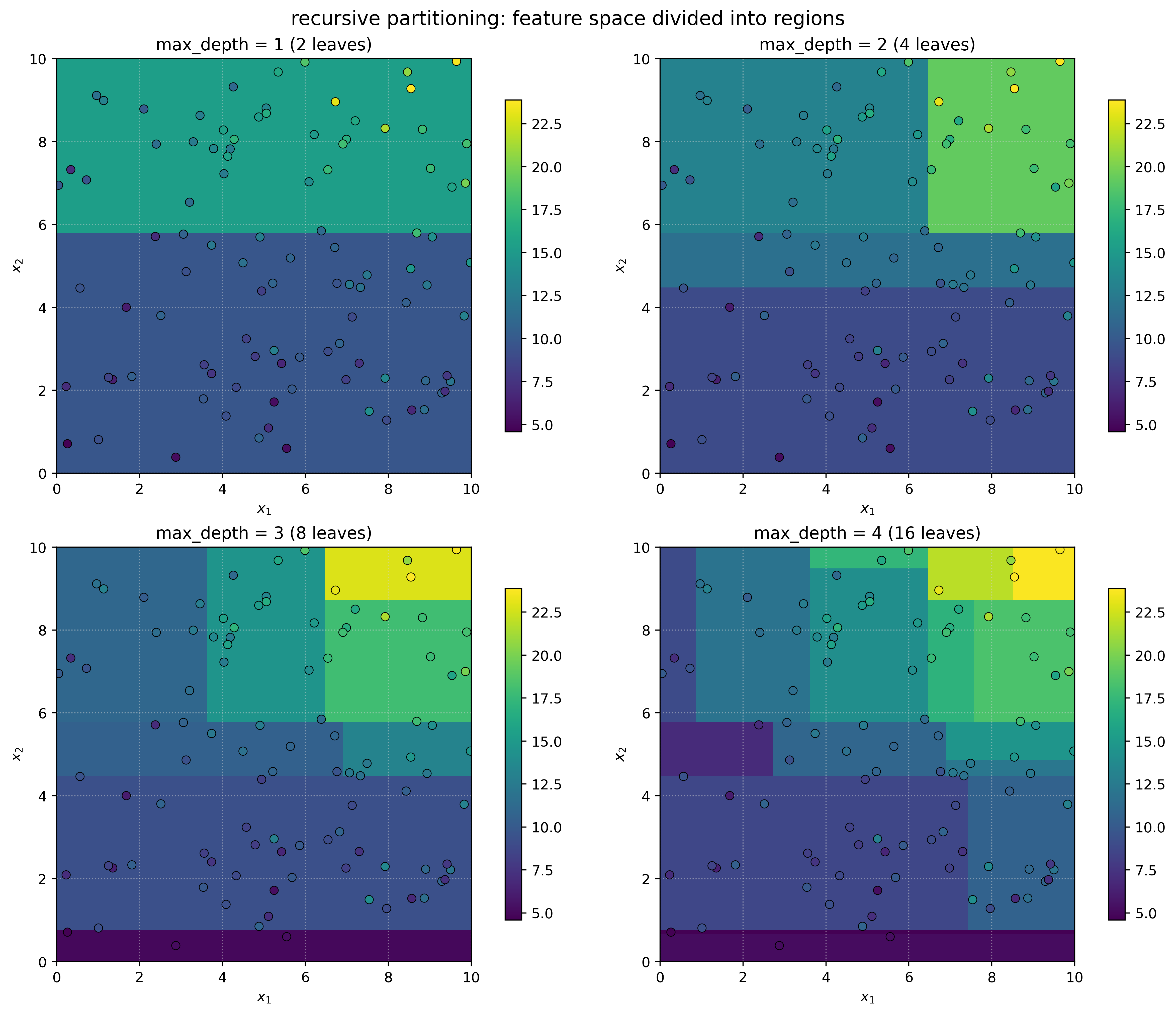
Example: Automobile Fuel Efficiency
auto_mpg = fetch_ucirepo("Auto MPG")We load the Auto MPG dataset using the fetch_ucirepo function, which provides access to datasets from the UCI Machine Learning Repository.
X = auto_mpg.data.features
y = auto_mpg.data.targets["mpg"]
X_train, X_test, y_train, y_test = train_test_split(
X,
y,
test_size=0.2,
random_state=42,
)DecisionTreeRegressor().get_params(){'ccp_alpha': 0.0,
'criterion': 'squared_error',
'max_depth': None,
'max_features': None,
'max_leaf_nodes': None,
'min_impurity_decrease': 0.0,
'min_samples_leaf': 1,
'min_samples_split': 2,
'min_weight_fraction_leaf': 0.0,
'monotonic_cst': None,
'random_state': None,
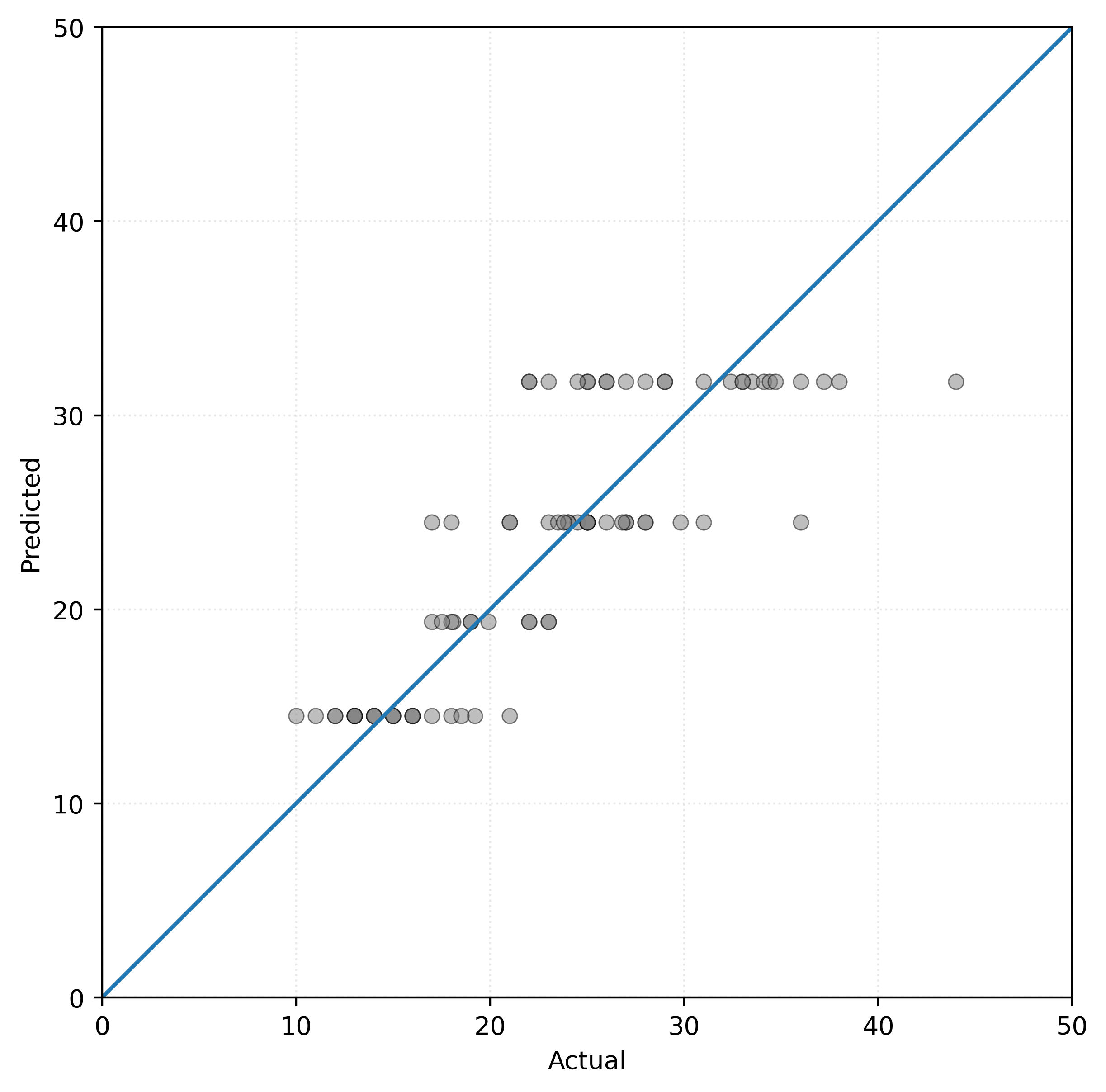
'splitter': 'best'}tree = DecisionTreeRegressor(max_depth=2, random_state=42)_ = tree.fit(X_train, y_train)tree.predict(X_test)array([31.7385, 31.7385, 19.3635, 14.5213, 14.5213, 24.4915, 24.4915,
14.5213, 19.3635, 14.5213, 14.5213, 31.7385, 31.7385, 14.5213,
31.7385, 14.5213, 24.4915, 24.4915, 14.5213, 31.7385, 31.7385,
19.3635, 19.3635, 31.7385, 14.5213, 31.7385, 24.4915, 24.4915,
19.3635, 14.5213, 24.4915, 31.7385, 19.3635, 24.4915, 31.7385,
14.5213, 24.4915, 14.5213, 14.5213, 31.7385, 24.4915, 31.7385,
24.4915, 14.5213, 24.4915, 24.4915, 31.7385, 24.4915, 24.4915,
31.7385, 31.7385, 31.7385, 31.7385, 14.5213, 24.4915, 14.5213,
14.5213, 24.4915, 24.4915, 19.3635, 14.5213, 31.7385, 31.7385,
24.4915, 19.3635, 24.4915, 24.4915, 31.7385, 31.7385, 14.5213,
31.7385, 14.5213, 14.5213, 19.3635, 24.4915, 19.3635, 19.3635,
24.4915, 31.7385, 14.5213])fig, ax = plt.subplots()
plot_tree(tree, feature_names=X_train.columns, filled=True, rounded=True)
plt.show()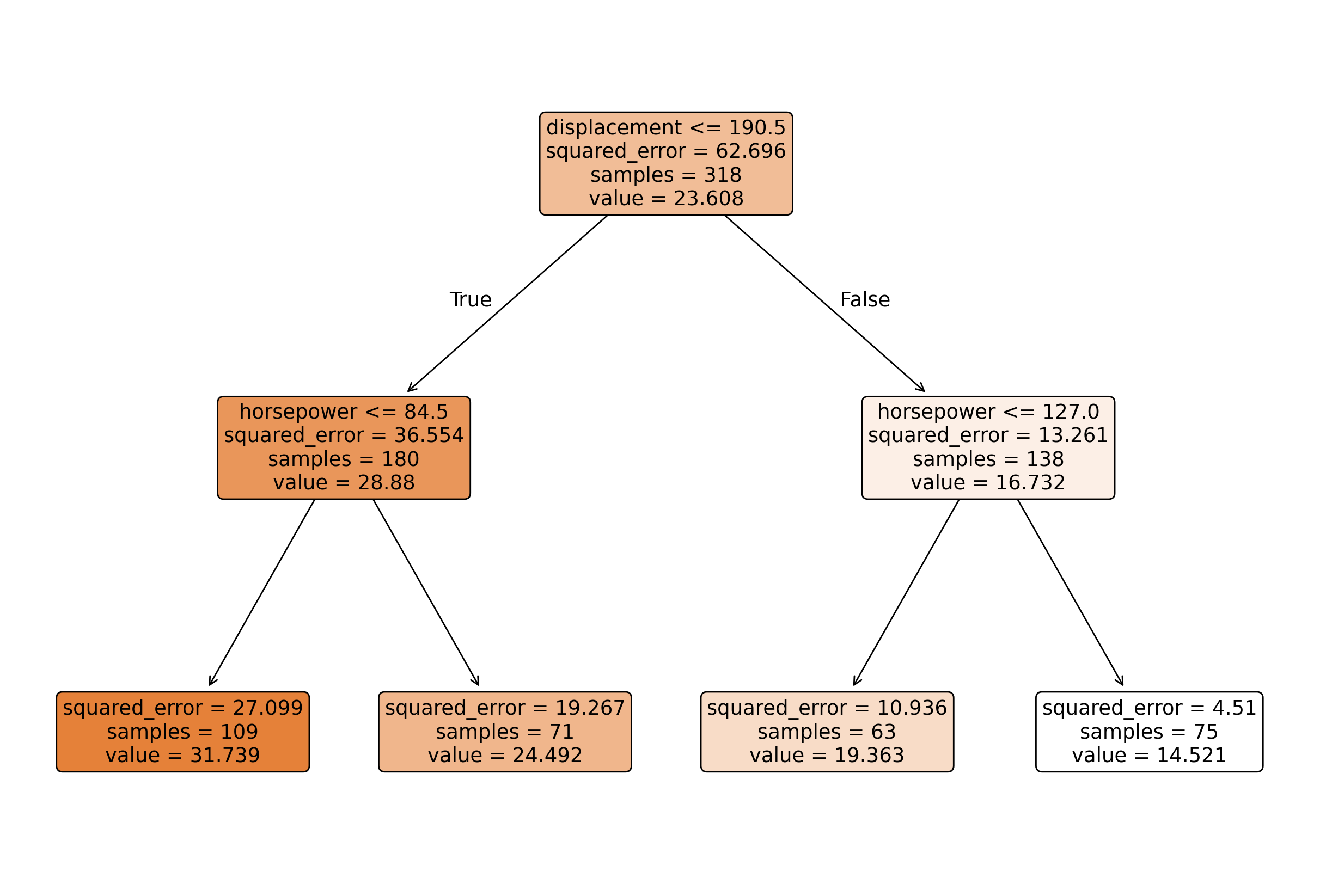
print(export_text(tree, feature_names=list(X_train.columns)))|--- displacement <= 190.50
| |--- horsepower <= 84.50
| | |--- value: [31.74]
| |--- horsepower > 84.50
| | |--- value: [24.49]
|--- displacement > 190.50
| |--- horsepower <= 127.00
| | |--- value: [19.36]
| |--- horsepower > 127.00
| | |--- value: [14.52]
Show Code for Plot
# setup figure
fig, ax = plt.subplots(figsize=(6, 6))

# create scatterplot
ax.scatter(y_test, tree.predict(X_test), alpha=0.50, c="tab:gray")
ax.axline((0, 0), slope=1)
ax.set_xlim(0, 50)
ax.set_ylim(0, 50)
ax.set_xlabel("Actual")
ax.set_ylabel("Predicted")
ax.set_aspect("equal")

# show figure
plt.show()