Classifier Calibration

Evaluating Probability Estimates

Table of Contents

• Objectives
• Python Setup
• Metrics
• Reliability Diagrams
• Calibrating a Classifier
• Calibration Methods
• Tuning and Calibrating
  • Data
  • No Tuning, No Calibration
  • No Tuning, Calibration
  • Tuning with Accuracy, Calibration
  • Tuning with Brier Score, Calibration
  • Tuning with ECE, Calibration
• Additional Resources

Objectives

In this note, we will discuss:

• calibration metrics including log loss, Brier score, and expected calibration error,
• reliability diagrams for visualizing the calibration of classifiers,
• and calibration methods such as isotonic regression and sigmoid calibration.

We will close with a discussion of tuning classifiers when a well-calibrated classifier (rather than simply high predictive accuracy) is needed.

• Probability Calibration | sklearn User Guide

Python Setup

import numpy as np
import pandas as pd
import matplotlib.pyplot as plt
from sklearn.datasets import make_classification
from sklearn.model_selection import train_test_split
from sklearn.linear_model import LogisticRegression
from sklearn.metrics import accuracy_score
from sklearn.metrics import log_loss
from sklearn.metrics import brier_score_loss
from sklearn.calibration import calibration_curve
from sklearn.calibration import CalibratedClassifierCV
from sklearn.ensemble import RandomForestClassifier
from sklearn.model_selection import GridSearchCV
from sklearn.metrics import make_scorer

Metrics

Given data with:

• \(n\), the number of samples
• \(y\), the vector of true target values
  • \(y_i\) is the true label of the \(i\)th sample
  • \(y_i \in \{0, 1\}\)
• \(p\), the vector of probabilities that \(y_i = 1\) given \(x_i\)
  • \(p_i\) is the probability for the \(i\)th sample
  • \(p_i \in [0, 1]\)

We can define two metrics to evaluate the performance of a (binary) classifier:

Log Loss

\[ \text{LogLoss}(y, p) = -\frac{1}{n} \sum_{i=1}^{n} \left[ y_i \log(p_i) + (1 - y_i) \log(1 - p_i) \right] \]

Brier Score

\[ \text{BrierScore}(y, p) = \frac{1}{n} \sum_{i=1}^{n} (y_i - p_i)^2 \]

# simulate data for binary classification
X, y = make_classification(
    n_samples=5000,
    n_features=4,
    n_classes=2,
    random_state=1,
)

X[:10]

array([[ 0.028 ,  0.7405,  0.5971,  0.3176],
       [-0.1771,  0.3478,  0.4024, -0.1792],
       [-0.5297, -0.714 , -0.2537, -1.1738],
       [-1.5094,  3.0382,  3.4909, -1.5006],
       [-1.428 ,  1.4334,  2.1056, -1.9436],
       [ 1.9512, -1.411 , -2.4223,  2.8549],
       [ 0.9372, -1.8126, -2.1062,  0.9586],
       [ 0.4968, -1.6762, -1.7107,  0.2482],
       [-0.8023, -0.6586, -0.0331, -1.6242],
       [-0.5237,  0.9684,  1.14  , -0.5519]])

y[:10]

array([1, 0, 0, 1, 1, 0, 0, 0, 0, 1])

np.mean(y)

np.float64(0.4996)

# train-test split the data
X_train, X_test, y_train, y_test = train_test_split(
    X,
    y,
    test_size=0.2,
    random_state=42,
)

# create and fit logistic regression model
model = LogisticRegression(random_state=42)
model.fit(X_train, y_train)

LogisticRegression(random_state=42)

In a Jupyter environment, please rerun this cell to show the HTML representation or trust the notebook.
On GitHub, the HTML representation is unable to render, please try loading this page with nbviewer.org.

# get predicted probabilities and classification
y_pred_proba = model.predict_proba(X_test)[:, 1]
y_pred = model.predict(X_test)

# calculate metrics
test_accuracy = accuracy_score(y_test, y_pred)
test_logloss = log_loss(y_test, y_pred_proba)
test_brier_score = brier_score_loss(y_test, y_pred_proba)
print(f"Test Accuracy: {test_accuracy:.4f}")
print(f"Log Loss: {test_logloss:.4f}")
print(f"Brier Score: {test_brier_score:.4f}")

Test Accuracy: 0.8770
Log Loss: 0.3116
Brier Score: 0.0941

# function to calculate the calibration error
def calibration_error(y_true, y_prob, type="expected", n_bins=10):
    """
    Compute calibration error of a binary classifier.

    The calibration error measures the aggregated difference between
    the average predicted probabilities assigned to the positive class,
    and the frequencies of the positive class in the actual outcome.

    Parameters
    ----------
    y_true : array-like of shape (n_samples,)
        True targets of a binary classification task.

    y_prob : array-like of (n_samples,)
        Estimated probabilities for the positive class.

    type : {'expected', 'max'}, default='expected'
        The expected-type is the Expected Calibration Error (ECE), and the
        max-type corresponds to Maximum Calibration Error (MCE).

    n_bins : int, default=10
       The number of bins used when computing the error.

    Returns
    -------
    score : float
        The calibration error.
    """

    bins = np.linspace(0.0, 1.0, n_bins + 1)
    bin_idx = np.searchsorted(bins[1:-1], y_prob)

    bin_sums = np.bincount(bin_idx, weights=y_prob, minlength=len(bins))
    bin_true = np.bincount(bin_idx, weights=y_true, minlength=len(bins))
    bin_total = np.bincount(bin_idx, minlength=len(bins))

    nonzero = bin_total != 0
    prob_true = bin_true[nonzero] / bin_total[nonzero]
    prob_pred = bin_sums[nonzero] / bin_total[nonzero]

    if type == "max":
        calibration_error = np.max(np.abs(prob_pred - prob_true))
    elif type == "expected":
        bin_error = np.abs(prob_pred - prob_true) * bin_total[nonzero]
        calibration_error = np.sum(bin_error) / len(y_true)

    return calibration_error

Expected Calibration Error (ECE)

\[ \text{ECE}(y, p) = \sum_{m=1}^M \frac{|B_m|}{n} | \bar{y}(B_m) - \bar{p}(B_m) | \]

Maximum Calibration Error (MCE)

\[ \text{MCE}(y, p) = \max_m | \bar{y}(B_m) - \bar{p}(B_m) | \]

• \(n\), the number of samples
• \(y\), the vector of true labels
• \(p\), the vector of (usually estimated) probabilities that \(y_i = 1\) given \(x_i\)
• \(M\), the number of bins
• \(|B_m|\), the number of samples in the \(m\)th bin
• \(\bar{y}(B_m)\), the proportion of samples in the \(m\)th bin with \(y_i = 1\)
  • \(\bar{y}(B_m) = \frac{1}{|B_m|} \displaystyle\sum_{i \in B_m} y_i\)
• \(\bar{p}(B_m)\), the average probability in the \(m\)th bin
  • \(\bar{p}(B_m) = \frac{1}{|B_m|} \displaystyle\sum_{i \in B_m} p_i\)

test_ece = calibration_error(
    y_test,
    y_pred_proba,
    type="expected",
)
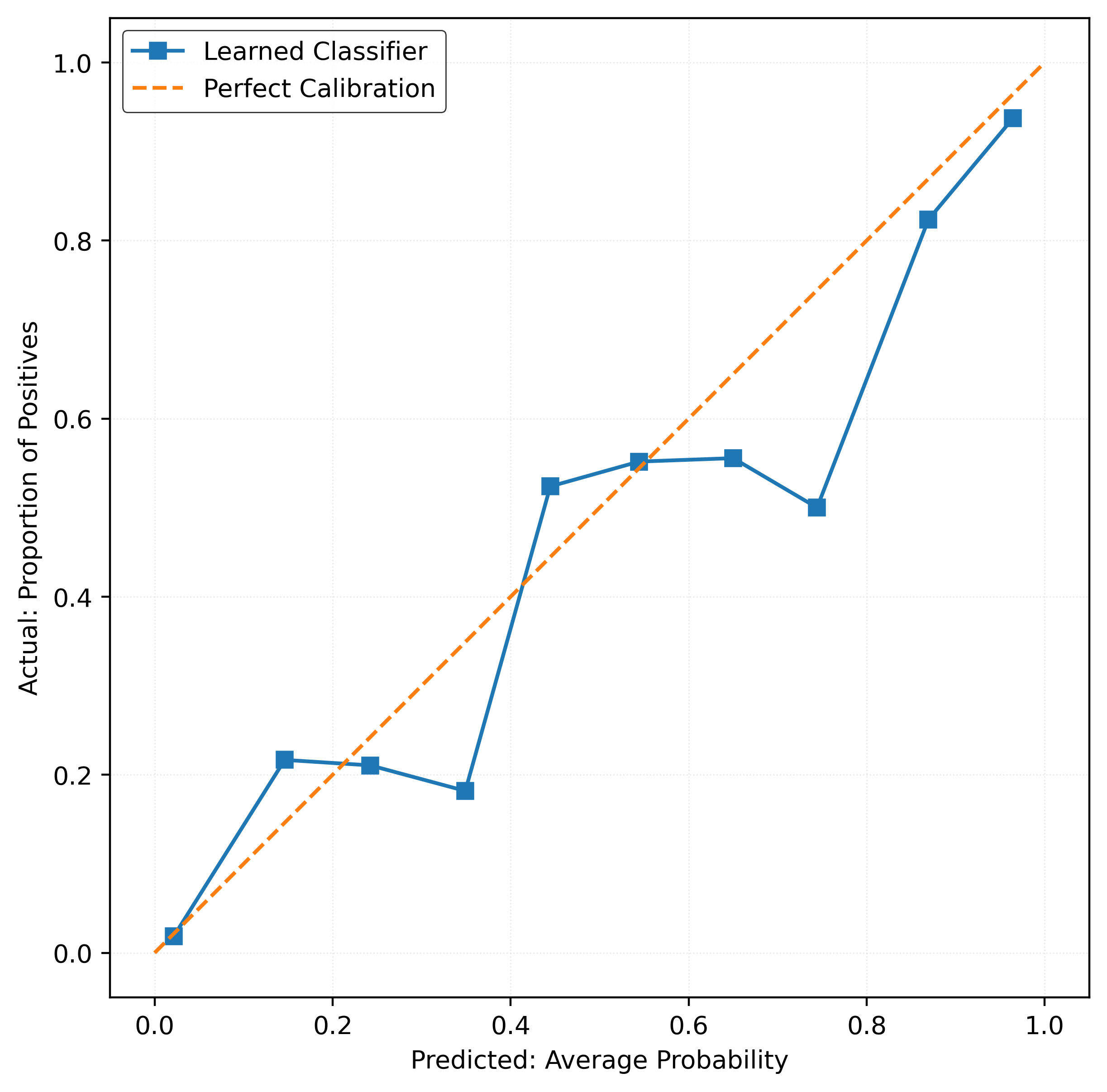
print(f"Test ECE: {test_ece:.4f}")

Test ECE: 0.0351

Reliability Diagrams

# function to plot a reliability diagram
def plot_reliability_diagram(y_true, y_prob):

    # generate "data" for reliability diagram
    prob_true, prob_pred = calibration_curve(
        y_true,
        y_prob,
        n_bins=10,
        pos_label=1,
    )

    # create a figure and axis object with a specific size
    fig, ax = plt.subplots(figsize=(6, 6))

    # plot the reliability diagram
    ax.plot(
        prob_pred,
        prob_true,
        "s-",
        label="Learned Classifier",
        color="tab:blue",
    )

    # plot the diagonal "perfect" line
    ax.plot(
        [0, 1],
        [0, 1],
        "--",
        label="Perfect Calibration",
        color="tab:orange",
    )

    # set the plot title and axis labels
    ax.set_xlabel("Predicted: Average Probability")
    ax.set_ylabel("Actual: Proportion of Positives")

    # add a grid
    ax.grid(
        True,
        color="lightgrey",
        linewidth=0.5,
        linestyle=":",
    )

    # fix aspect ratio
    ax.set_aspect("equal")

    # show the legend
    ax.legend()

    # show the plot
    plt.show()

plot_reliability_diagram(y_test, y_pred_proba)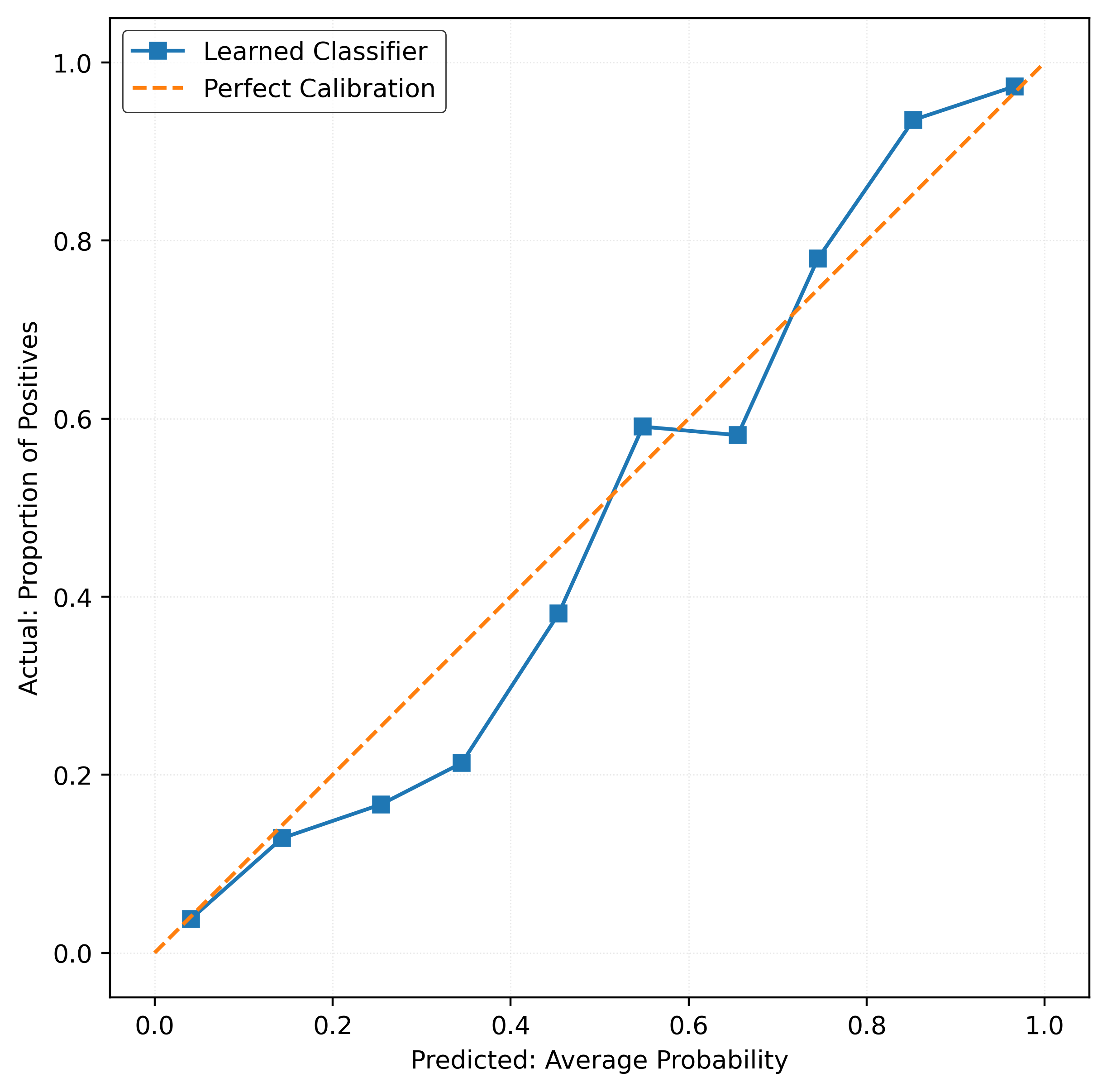

Calibrating a Classifier

# create a calibrated model
model_calibrated = CalibratedClassifierCV(
    estimator=LogisticRegression(random_state=42),
    method="isotonic",
)
model_calibrated.fit(X_train, y_train)

CalibratedClassifierCV(estimator=LogisticRegression(random_state=42),
                       method='isotonic')

In a Jupyter environment, please rerun this cell to show the HTML representation or trust the notebook.
On GitHub, the HTML representation is unable to render, please try loading this page with nbviewer.org.

# get predicted probabilities and classification
y_pred_proba_calibrated = model_calibrated.predict_proba(X_test)[:, 1]
y_pred_calibrated = model_calibrated.predict(X_test)

# calculate metrics
test_accuracy_calibrated = accuracy_score(y_test, y_pred_calibrated)
test_logloss_calibrated = log_loss(y_test, y_pred_proba_calibrated)
test_brier_score_calibrated = brier_score_loss(y_test, y_pred_proba_calibrated)
print(f"Calibrated Test Accuracy: {test_accuracy_calibrated:.4f}")
print(f"Calibrated Log Loss: {test_logloss_calibrated:.4f}")
print(f"Calibrated Brier Score: {test_brier_score_calibrated:.4f}")

Calibrated Test Accuracy: 0.8780
Calibrated Log Loss: 0.3077
Calibrated Brier Score: 0.0932

test_ece_calibrated = calibration_error(
    y_test,
    y_pred_proba_calibrated,
    type="expected",
)
print(f"Test ECE: {test_ece_calibrated:.4f}")

Test ECE: 0.0208

plot_reliability_diagram(y_test, y_pred_proba_calibrated)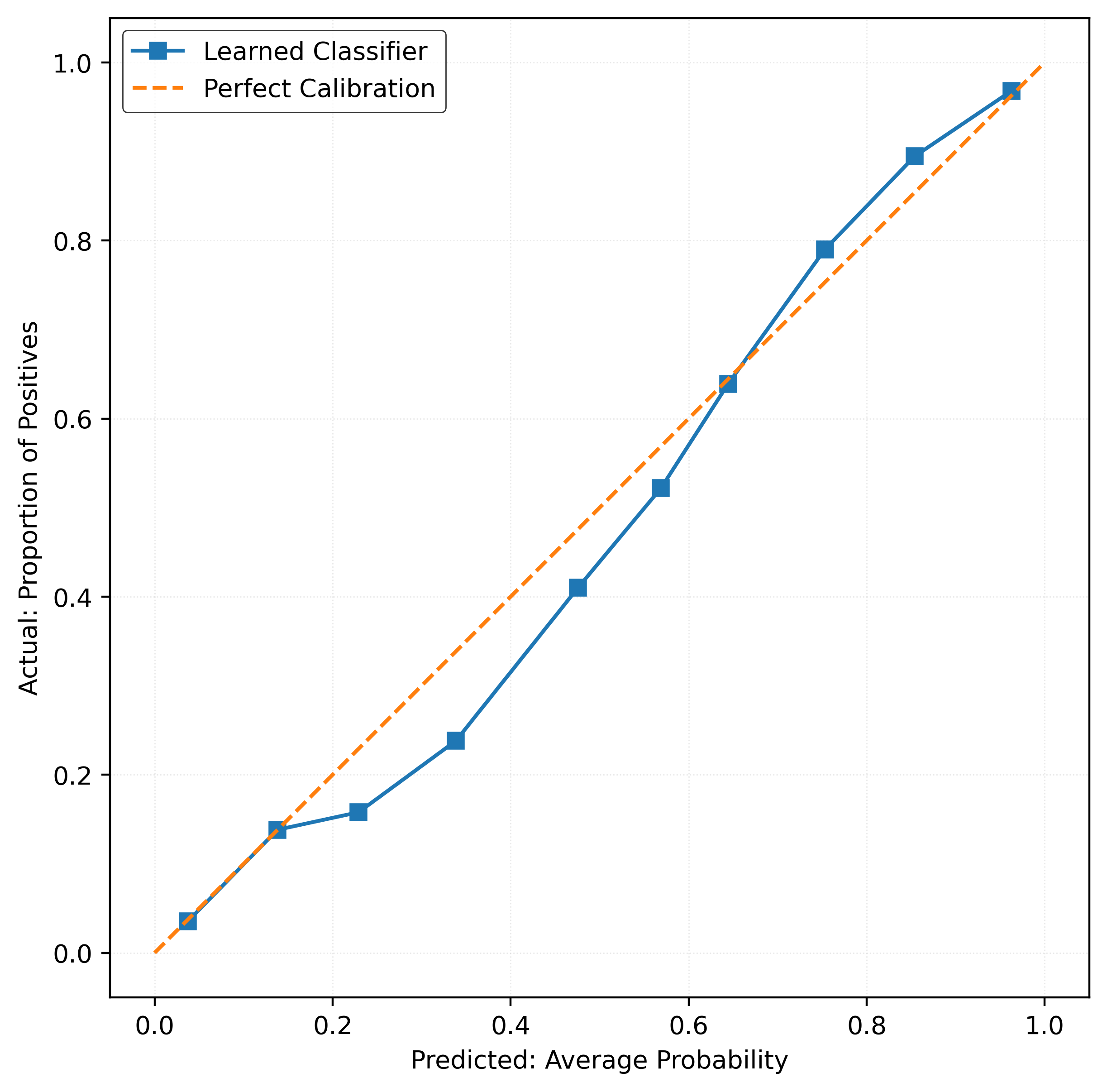

Calibration Methods

When a classifier produces poorly-calibrated probability estimates, we can apply post-hoc calibration methods to improve them. The sklearn package provides two primary calibration approaches through the CalibratedClassifierCV class:

Sigmoid Calibration

Sigmoid calibration (also known as Platt scaling) fits a logistic regression model on top of the classifier’s predicted probabilities. This method assumes that the mis-calibration can be corrected by applying a sigmoid function to transform the original probabilities:

\[ p_{\text{calibrated}} = \frac{1}{1 + \exp(A \cdot p_{\text{original}} + B)} \]

where \(A\) and \(B\) are parameters learned from a calibration set. This approach works well when the calibration curve has a sigmoid shape and is particularly effective for models that tend to push probabilities toward 0 or 1.

Isotonic Regression

Isotonic regression is a non-parametric method that fits a piecewise-constant, monotonically increasing function to map original probabilities to calibrated ones. Unlike sigmoid calibration, it makes no assumptions about the functional form of the mis-calibration and can correct more complex calibration patterns. However, it is more prone to overfitting, especially with smaller calibration datasets, since it has more flexibility to fit the data.

Both methods require a held-out calibration dataset. When using CalibratedClassifierCV, this is handled automatically through cross-validation, ensuring that the calibration is performed on data not used for training the base classifier.

Tuning and Calibrating

Data

X, y = make_classification(
    n_samples=2000,
    n_features=20,
    n_informative=2,
    n_redundant=2,
    class_sep=0.90,
    random_state=42,
)

X_train, X_test, y_train, y_test = train_test_split(
    X,
    y,
    test_size=0.5,
    random_state=42,
)

No Tuning, No Calibration

mod = RandomForestClassifier(
    n_estimators=25,
    random_state=42,
)
mod.fit(X_train, y_train)
y_pred_proba = mod.predict_proba(X_test)[:, 1]

calibration_error(y_test, y_pred_proba)

np.float64(0.03303999999999967)

plot_reliability_diagram(y_test, y_pred_proba)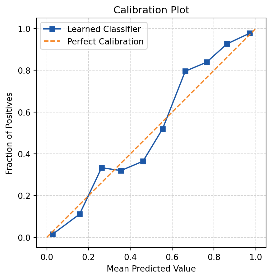

No Tuning, Calibration

mod = CalibratedClassifierCV(
    estimator=RandomForestClassifier(
        n_estimators=25,
        random_state=42,
    ),
    method="sigmoid",
)
mod.fit(X_train, y_train)
y_pred_proba = mod.predict_proba(X_test)[:, 1]

calibration_error(y_test, y_pred_proba)

np.float64(0.025660079499866723)

plot_reliability_diagram(y_test, y_pred_proba)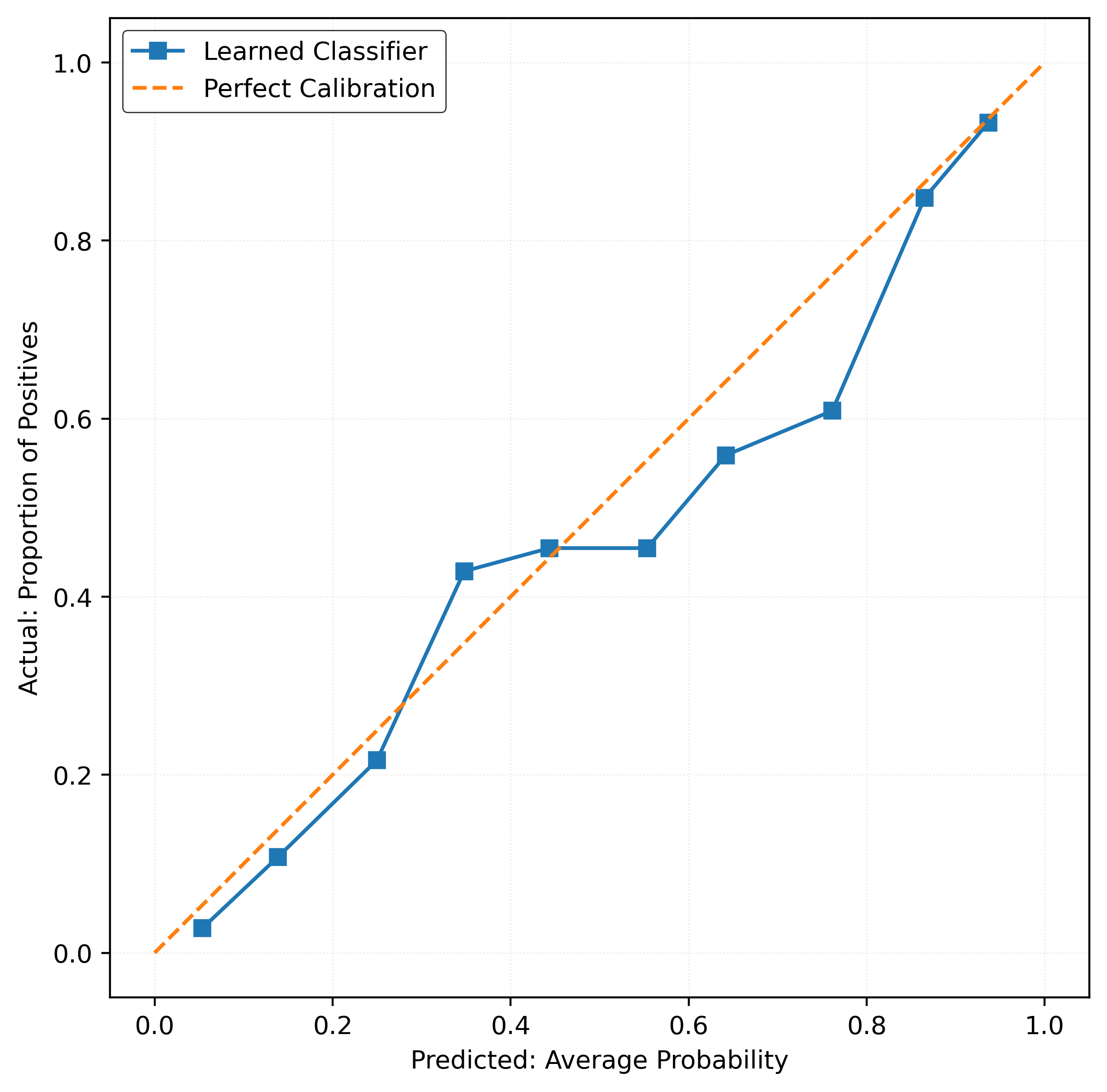

Tuning with Accuracy, Calibration

params_grid = {
    "method": [
        "isotonic",
        "sigmoid",
    ],
    "estimator__max_depth": [5, 10, 15, 25, None],
    "estimator__criterion": ["log_loss", "gini"],
}

mod = GridSearchCV(
    CalibratedClassifierCV(
        estimator=RandomForestClassifier(
            n_estimators=25,
            random_state=42,
        ),
    ),
    cv=5,
    param_grid=params_grid,
    n_jobs=-1,
)
mod.fit(X_train, y_train)
y_pred_proba = mod.predict_proba(X_test)[:, 1]

calibration_error(y_test, y_pred_proba)

np.float64(0.022058773218403237)

plot_reliability_diagram(y_test, y_pred_proba)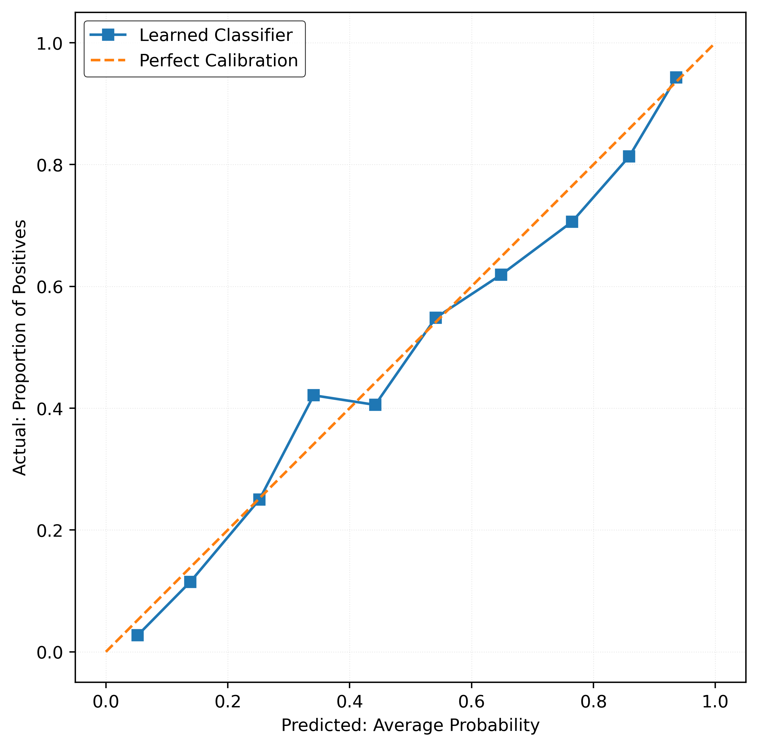

Tuning with Brier Score, Calibration

mod = GridSearchCV(
    CalibratedClassifierCV(
        estimator=RandomForestClassifier(
            n_estimators=25,
            random_state=42,
        ),
    ),
    cv=5,
    param_grid=params_grid,
    n_jobs=-1,
    scoring="neg_brier_score",
)
mod.fit(X_train, y_train)
y_pred_proba = mod.predict_proba(X_test)[:, 1]

calibration_error(y_test, y_pred_proba)

np.float64(0.022058773218403237)

plot_reliability_diagram(y_test, y_pred_proba)

Tuning with ECE, Calibration

# define a custom scoring function for ECE
def ece_scorer(y_true, y_prob):
    return -calibration_error(y_true, y_prob, type="expected", n_bins=10)

# create a scorer object for GridSearchCV
ece_scorer_func = make_scorer(ece_scorer, response_method="predict_proba")

mod = GridSearchCV(
    CalibratedClassifierCV(
        estimator=RandomForestClassifier(
            n_estimators=25,
            random_state=42,
        ),
    ),
    cv=5,
    param_grid=params_grid,
    n_jobs=-1,
    scoring=ece_scorer_func,
)
mod.fit(X_train, y_train)
y_pred_proba = mod.predict_proba(X_test)[:, 1]

calibration_error(y_test, y_pred_proba)

np.float64(0.03634713644017977)

plot_reliability_diagram(y_test, y_pred_proba)

Additional Resources

• When Calibration Beats Metrics | YouTube
• How to Remedy a Badly Calibrated Machine Learning Model | YouTube
• Classifier Calibration: A Survey on How to Assess and Improve Predicted Class Probabilities
• On Calibration of Modern Neural Networks
• Model Agnostic Prediction Interval Estimator

TODO

• https://jonathanwenger.github.io/pycalib/_modules/pycalib/scoring.html#expected_calibration_error
• what is a confidence?
• confidence version versus probability version (at least for binary classification)
• https://scikit-learn.org/stable/modules/calibration.html
• https://scikit-learn.org/stable/modules/generated/sklearn.calibration.CalibratedClassifierCV.html
• https://towardsdatascience.com/expected-calibration-error-ece-a-step-by-step-visual-explanation-with-python-code-c3e9aa12937d/

ece = calibration_error(y_test, mod.predict_proba(X_test)[:, 1], type="expected", n_bins=10)
print(f"Expected Calibration Error (ECE): {ece:.4f}")

Expected Calibration Error (ECE): 0.0363

from sklearn.metrics import make_scorer


# define a custom scoring function for ECE
def ece_scorer(y_true, y_prob):
    return -calibration_error(y_true, y_prob, type="expected", n_bins=10)


# create a scorer object for GridSearchCV
ece_scorer_func = make_scorer(ece_scorer, response_method="predict_proba")

# define the classifier
mod = GridSearchCV(
    CalibratedClassifierCV(
        estimator=RandomForestClassifier(
            n_estimators=25,
            random_state=42,
        ),
    ),
    cv=5,
    param_grid=params_grid,
    n_jobs=-1,
    scoring=ece_scorer_func,
)
mod.fit(X_train, y_train)
plot_reliability_diagram(y_test, mod.predict_proba(X_test)[:, 1])