# basics
import numpy as np
import pandas as pd
import matplotlib.pyplot as plt
import seaborn as sns
from scipy.stats import norm

# general machine Learning
from sklearn.datasets import make_blobs
from sklearn.datasets import make_classification
from sklearn.pipeline import Pipeline
from sklearn.linear_model import LogisticRegression
from sklearn.model_selection import train_test_split

# unsupervised learning
from sklearn.decomposition import PCA
from sklearn.cluster import KMeans
from sklearn.cluster import AgglomerativeClustering
from sklearn.cluster import DBSCAN
from sklearn.mixture import GaussianMixture
from sklearn.neighbors import KernelDensity
from sklearn.ensemble import IsolationForestUnsupervised Learning
Learning Without a Supervisor
Objectives
In this note, we will discuss unsupervised learning, including:
- dimension reduction using principal component analysis (PCA),
- clustering methods including K-Means, DBSCAN, and agglomerative clustering,
- density estimation with kernel density estimation and Gaussian mixture models,
- and outlier detection using isolation forests.
Python Setup
Introduction
Dimension Reduction
X, _ = make_blobs(
    n_samples=500,
    centers=4,
    n_features=50,
    cluster_std=5,
    random_state=42,
)
X
array([[ 5.4727, 2.3671, -7.728 , ..., 11.5627, 5.3876, 8.3044],
[ 1.8549, 4.1835, 4.2429, ..., 6.9523, -0.1456, -1.6155],
[ -4.8382, 8.2601, 4.2701, ..., 1.9069, 1.8534, 7.1623],
...,
[ 22.3216, 7.5979, 11.8563, ..., -7.0752, -14.9351, -5.0348],
[ 6.9927, -11.1958, -3.5367, ..., 7.5444, 17.3163, 0.1853],
[-13.9122, 0.6172, -4.8026, ..., -7.4577, -8.1849, -4.0837]],
shape=(500, 50))X.shape(500, 50)fig, ax = plt.subplots(figsize=(6, 4))
sns.scatterplot(
x=X[:, 0],
y=X[:, 1],
ax=ax,
)
ax.set_xlabel(r"$x_1$")
ax.set_ylabel(r"$x_2$")
plt.show()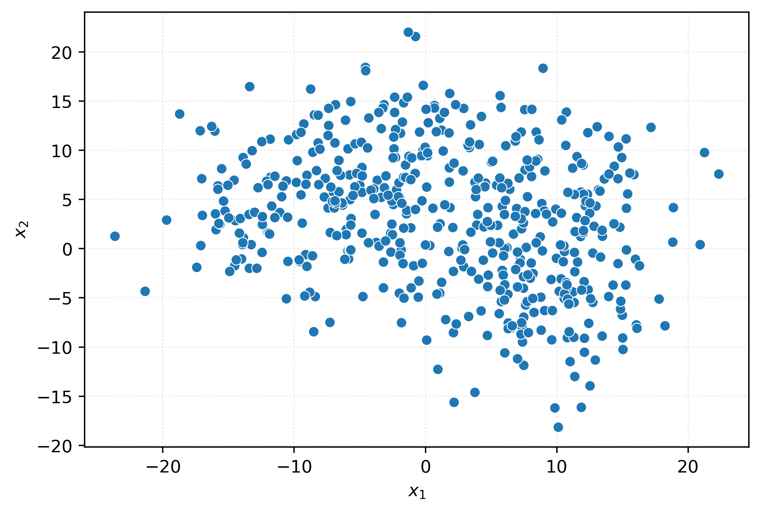
fig, ax = plt.subplots(figsize=(6, 4))
sns.scatterplot(
    x=X[:, 1],
    y=X[:, 2],
    ax=ax,
)
ax.set_xlabel(r"$x_2$")
ax.set_ylabel(r"$x_3$")
plt.show()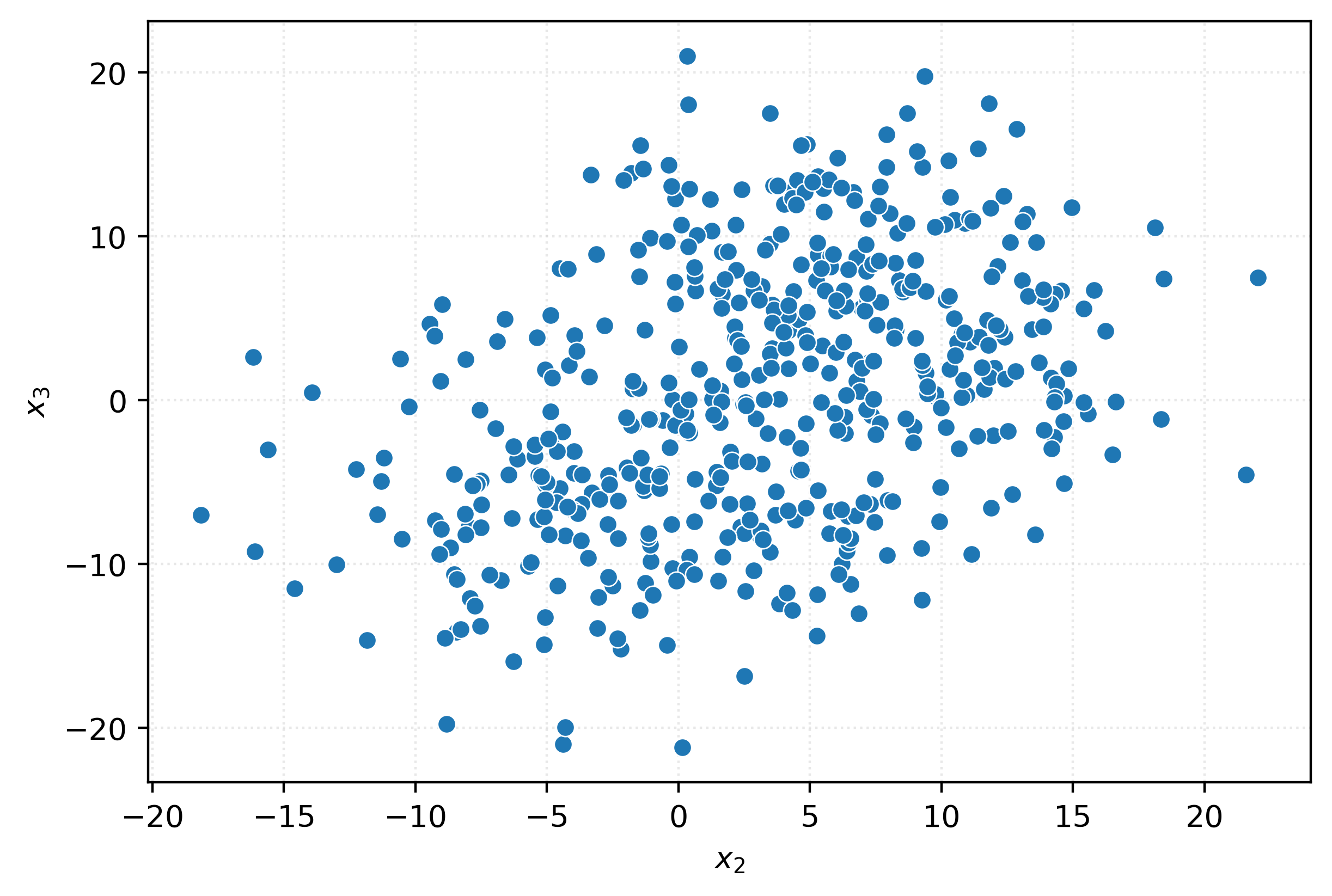
pca = PCA()
_ = pca.fit(X)
X_pca = pca.transform(X)
X_pca
array([[-21.0132, 0.5843, -18.7813, ..., -3.4356, -3.4878, 7.135 ],
[ -8.294 , 41.0983, 20.5115, ..., -0.6895, -6.5105, 2.5496],
[ -6.552 , 30.9882, 9.6581, ..., 1.2333, 3.8608, 0.8317],
...,
[-14.2974, -37.3181, 36.2534, ..., 2.1426, 1.0694, -2.0534],
[-20.7484, 2.0195, -37.9458, ..., -0.7764, 4.3229, -3.0478],
[ 43.9207, -2.5728, -8.6172, ..., -1.6524, -9.0256, 6.9946]],
shape=(500, 50))X_pca[:10, :3]array([[-21.0132, 0.5843, -18.7813],
[ -8.294 , 41.0983, 20.5115],
[ -6.552 , 30.9882, 9.6581],
[ 44.2098, -10.112 , 1.6899],
[ 38.057 , -14.7039, -11.5185],
[ 41.837 , 1.7666, -8.2681],
[ 24.5627, -0.9031, -8.599 ],
[ -5.6833, 26.3051, 10.748 ],
[ -3.1338, 27.507 , 12.3295],
[ 47.819 , -8.8634, -9.2638]])X_pca.shape(500, 50)fig, ax = plt.subplots(figsize=(6, 4))
sns.scatterplot(
x=X_pca[:, 0],
y=X_pca[:, 1],
ax=ax,
)
ax.set_xlabel("Principal Component 1")
ax.set_ylabel("Principal Component 2")
plt.show()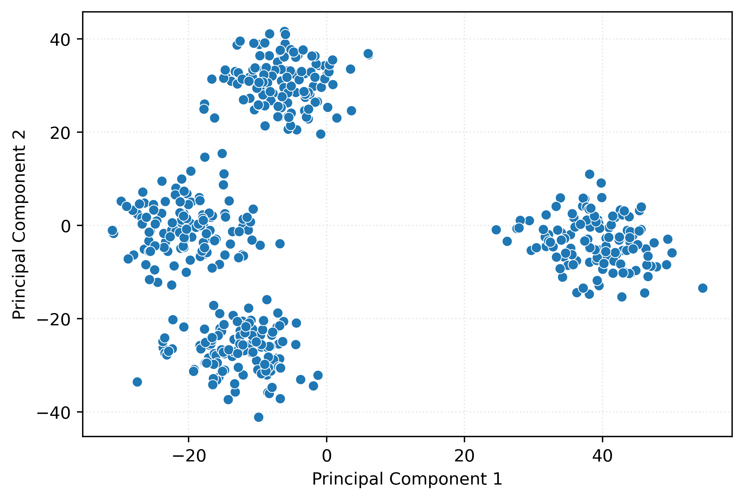
fig, ax = plt.subplots(figsize=(6, 4))
sns.scatterplot(
    x=X_pca[:, 1],
    y=X_pca[:, 2],
    ax=ax,
)
ax.set_xlabel("Principal Component 2")
ax.set_ylabel("Principal Component 3")
plt.show()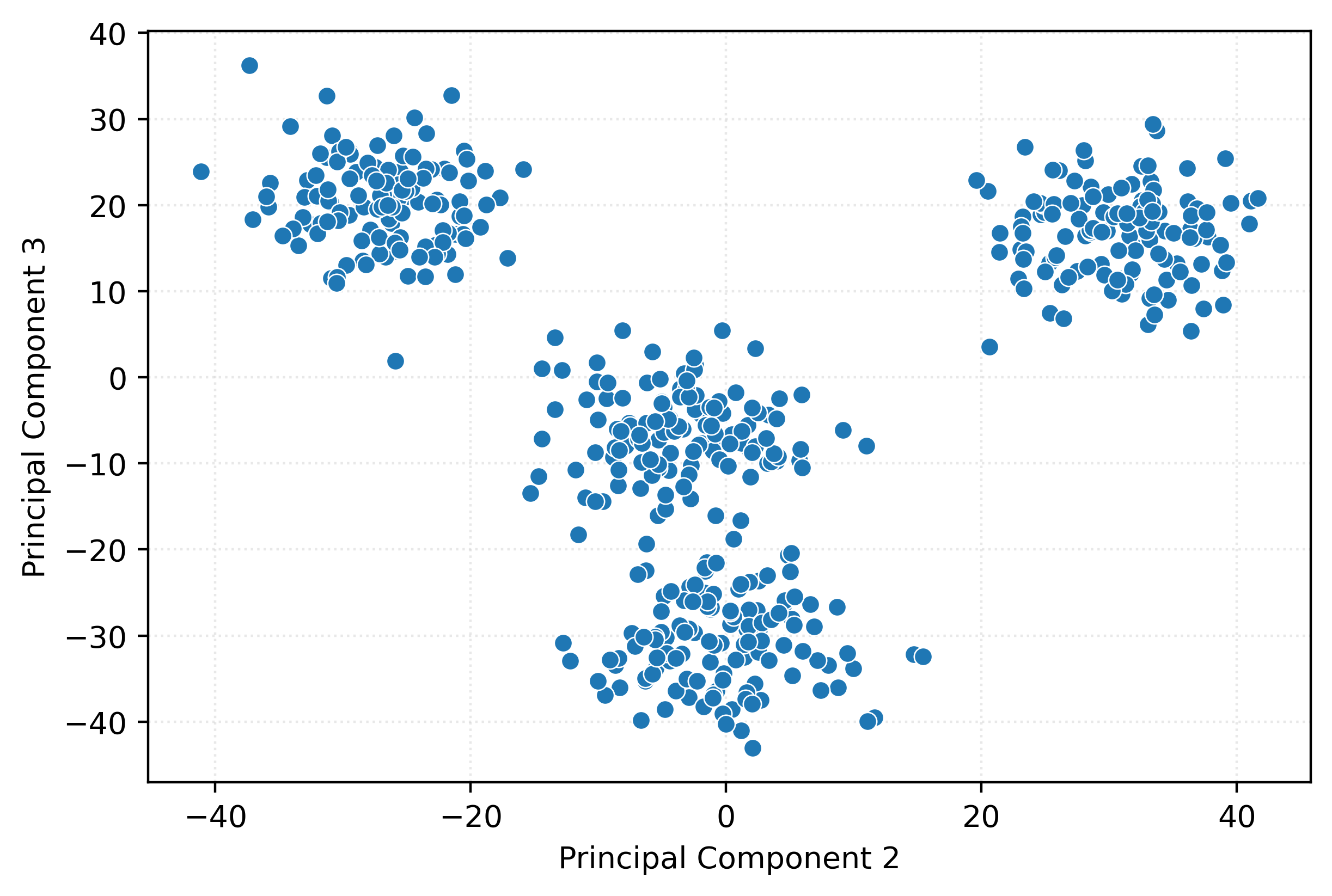
fig, ax = plt.subplots(figsize=(6, 4))
sns.scatterplot(
    x=X_pca[:, 2],
    y=X_pca[:, 3],
    ax=ax,
)
ax.set_xlabel("Principal Component 3")
ax.set_ylabel("Principal Component 4")
plt.show()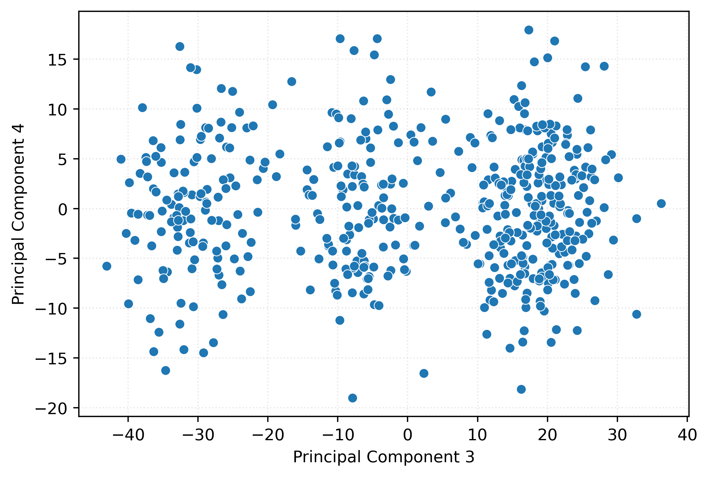
fig, ax = plt.subplots(figsize=(6, 4))
sns.scatterplot(
    x=X_pca[:, 9],
    y=X_pca[:, 10],
    ax=ax,
)
ax.set_xlabel("Principal Component 10")
ax.set_ylabel("Principal Component 11")
plt.show()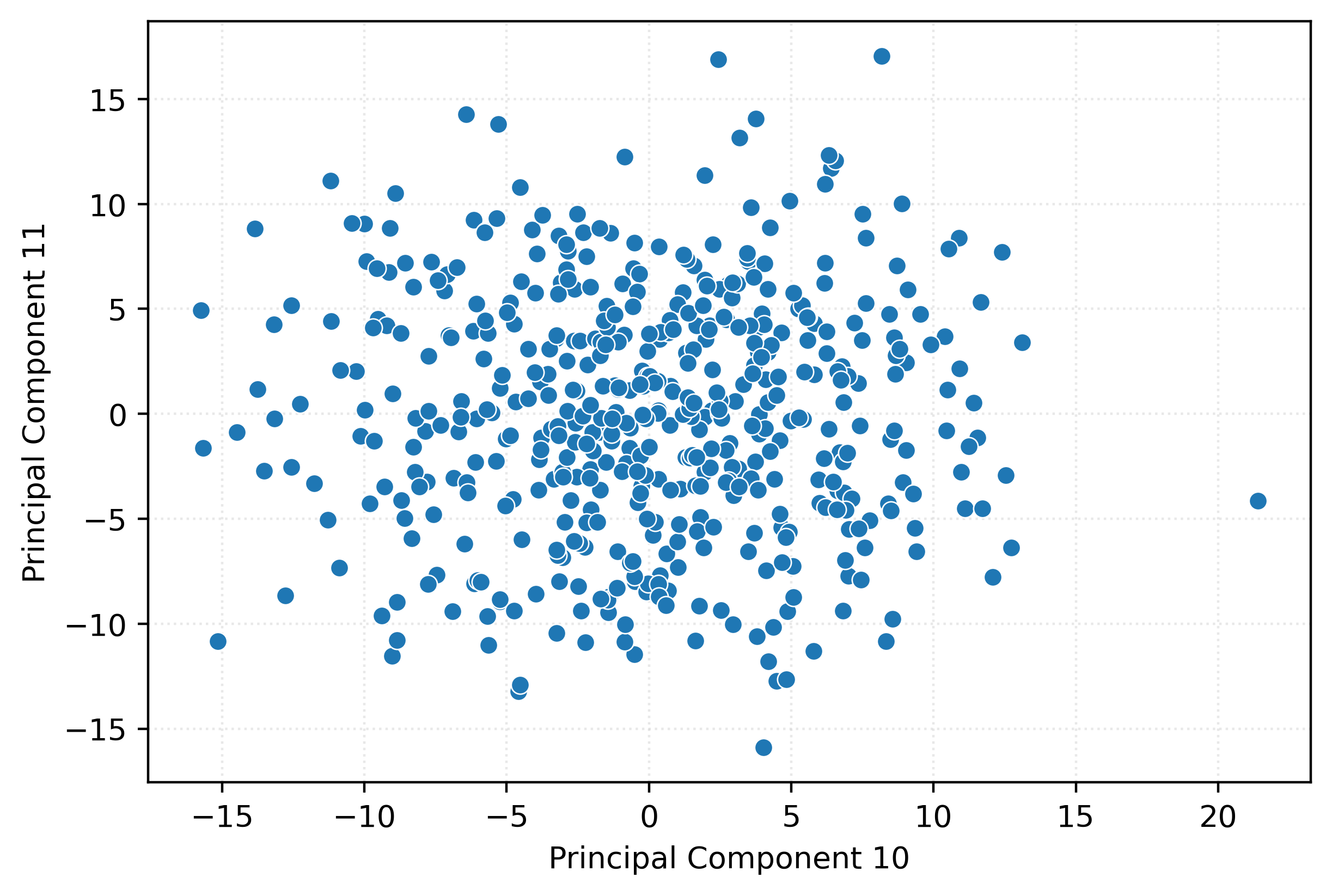
# center the data
X_centered = X - np.mean(X, axis=0)

# compute the covariance matrix
cov_matrix = np.cov(X_centered, rowvar=False)

# compute the eigenvalues and eigenvectors
eigenvalues, eigenvectors = np.linalg.eigh(cov_matrix)

# sort the eigenvectors by eigenvalues in descending order
sorted_indices = np.argsort(eigenvalues)[::-1]
eigenvectors = eigenvectors[:, sorted_indices]

# project the data
X_pca_numpy = np.dot(X_centered, eigenvectors)

# print the first 10 rows of the first three principal components
X_pca_numpy[:10, :3]
array([[-21.0132, -0.5843, -18.7813],
[ -8.294 , -41.0983, 20.5115],
[ -6.552 , -30.9882, 9.6581],
[ 44.2098, 10.112 , 1.6899],
[ 38.057 , 14.7039, -11.5185],
[ 41.837 , -1.7666, -8.2681],
[ 24.5627, 0.9031, -8.599 ],
[ -5.6833, -26.3051, 10.748 ],
[ -3.1338, -27.507 , 12.3295],
[ 47.819 , 8.8634, -9.2638]])np.allclose(X_pca[:,:1], X_pca_numpy[:,:1])Truenp.allclose(X_pca[:,1:2], -X_pca_numpy[:,1:2])Truepca = PCA(n_components=2)
_ = pca.fit(X)
X_pca = pca.transform(X)
X_pca.shape(500, 2)pca = PCA(n_components=0.95)
_ = pca.fit(X)
X_pca = pca.transform(X)
X_pca.shape(500, 42)# create a synthetic dataset
X, y = make_classification(
n_samples=1000,
n_features=50,
n_informative=10,
n_redundant=10,
random_state=42,
)
# split into train and test sets
X_train, X_test, y_train, y_test = train_test_split(
X,
y,
test_size=0.2,
random_state=42,
)
# create and fit logistic regression
logistic = LogisticRegression(max_iter=1000, random_state=42)
logistic.fit(X_train, y_train)
# evaluate the logistic regression
accuracy = logistic.score(X_test, y_test)
print(f"Test Accuracy without PCA: {accuracy:.2f}")
# create a pipeline with PCA and Logistic Regression
pipeline = Pipeline(
[
("pca", PCA(n_components=10)),
("classifier", LogisticRegression(max_iter=1000, random_state=42)),
]
)
# fit the pipeline with PCA
pipeline.fit(X_train, y_train)
# evaluate the pipeline with PCA
accuracy_with_pca = pipeline.score(X_test, y_test)
print(f"Test Accuracy with PCA: {accuracy_with_pca:.2f}")Test Accuracy without PCA: 0.80
Test Accuracy with PCA: 0.82Clustering
K-Means
To fit \(K\)-Means, minimize the cost function, otherwise known as the within cluster sum of squares:
\[ C(\pmb x_i, \pmb\mu_1, \ldots, \pmb\mu_K, \pmb r_1, \ldots, \pmb r_K) = \sum_{i = 1}^{n}\sum_{k = 1}^{K} r_{ik} || \pmb x_i - \pmb\mu_k || ^ 2 \]
The responsibilities, \(r_{ik}\), are defined as:
\[ r_{ik} = \begin{cases} 1 & \text{if } \pmb x_i \text{ is closest to } \pmb\mu_k\\ 0 & \text{otherwise} \end{cases} \]
This means that \(r_{ik}\) is 1 if the center of cluster \(k\) is the closest to data point \(x_i\), and 0 otherwise.
Assuming \(\pmb x_i\) is a \(p\)-dimensional vector, we have:
\[ || \pmb x_i - \pmb\mu_k || ^ 2 = (x_{i1} - \mu_{k1}) ^ 2 + \ldots + (x_{ip} - \mu_{kp}) ^ 2. \]
This quantity is the squared Euclidean distance (also known as the L2 norm) between data point \(\pmb x_i\) and the center of cluster \(k\), \(\pmb\mu_k\). It measures the “closeness” of \(\pmb x_i\) to \(\pmb \mu_k\). The goal of \(K\)-Means is to minimize this distance for all data points and their assigned clusters, hence minimizing the within cluster sum of squares.
This is easy! Simply… assign each data point to its own cluster! But that is silly and useless. So instead, we will use the Expectation–Maximization (EM) Algorithm to fit \(K\)-Means, after first choosing a value of \(K\).
To perform \(K\)-Means, first choose \(K\), the number of clusters to learn. Initialize a random center for each cluster.
EM Algorithm for \(K\)-Means
- Pre-select a value of \(K\), then number of clusters to learn.
- Randomly initialize a center for each cluster.
- Repeat the E and M steps until convergence.
- E-Step: Update the responsibilities. That is, assign each data point to the cluster that has the closest center. \[ r_{ik} = \begin{cases} 1 & \text{if } \pmb x_i \text{ is closest to } \pmb\mu_k\\ 0 & \text{otherwise} \end{cases} \]
- If there are no updates to the responsibilities, the algorithm has converged.
- M-Step: Update the cluster centers \(\pmb \mu_k\) by calculating the mean of all data points assigned to cluster \(k\). \[ \mu_k = \frac{\sum_{i=1}^n r_{ik} \pmb x_i}{\sum_{i=1}^n r_{ik}} \]
Because of the random initialization, \(K\)-Means is often by default run multiples times, and the “best” outcome (the outcome with the lowest cost) is chosen.
X, _ = make_blobs(
    n_samples=500,
    n_features=2,
    cluster_std=1,
    random_state=3,
)
fig, ax = plt.subplots(figsize=(6, 4))
sns.scatterplot(
x=X[:, 0],
y=X[:, 1],
ax=ax,
)
ax.set_xlabel(r"$x_1$")
ax.set_ylabel(r"$x_2$")
plt.show()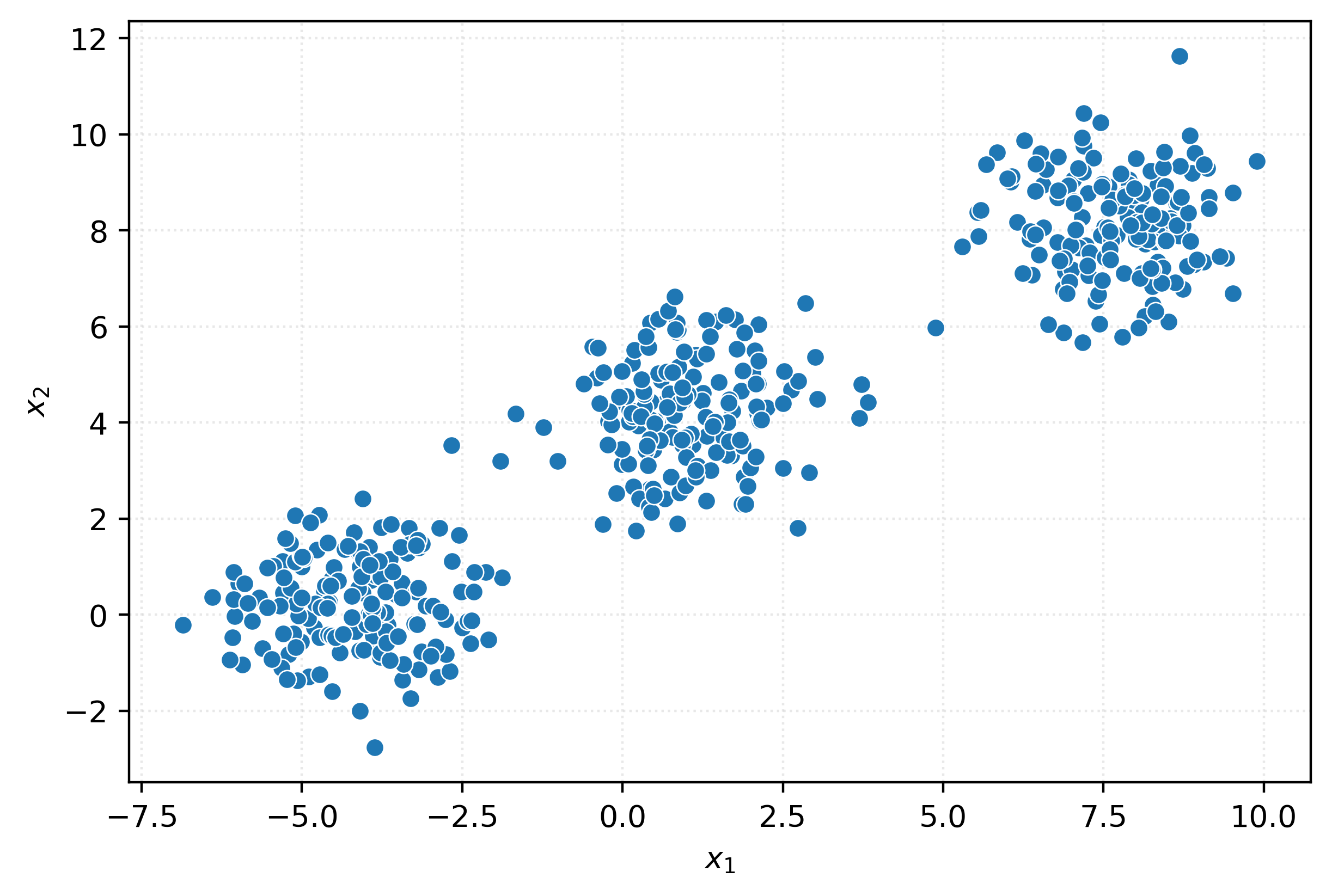
km = KMeans()
_ = km.fit(X)
clusters = km.predict(X)
clusters
array([5, 2, 6, 2, 0, 1, 4, 6, 0, 4, 2, 0, 4, 3, 0, 4, 6, 6, 7, 3, 2, 2,
6, 6, 3, 0, 1, 2, 3, 2, 2, 5, 2, 2, 2, 2, 2, 6, 3, 3, 1, 3, 1, 4,
2, 2, 2, 7, 6, 2, 6, 5, 6, 4, 2, 5, 0, 2, 4, 2, 6, 5, 7, 4, 2, 1,
3, 7, 2, 3, 2, 2, 6, 0, 2, 0, 4, 2, 2, 2, 0, 3, 2, 6, 7, 2, 2, 2,
0, 2, 1, 6, 5, 3, 4, 2, 3, 2, 2, 4, 0, 0, 2, 2, 4, 6, 3, 4, 0, 2,
2, 0, 2, 3, 1, 7, 1, 7, 2, 5, 7, 1, 7, 3, 4, 3, 3, 3, 2, 4, 3, 5,
5, 5, 7, 2, 3, 1, 2, 3, 4, 1, 0, 3, 6, 3, 2, 1, 6, 2, 5, 1, 2, 2,
1, 0, 4, 2, 4, 1, 2, 4, 2, 1, 2, 2, 2, 3, 7, 2, 7, 2, 3, 5, 2, 7,
5, 6, 3, 2, 3, 4, 2, 7, 2, 4, 2, 2, 1, 6, 1, 2, 6, 3, 0, 7, 0, 2,
2, 4, 7, 3, 3, 3, 6, 7, 3, 1, 2, 2, 1, 1, 3, 3, 2, 3, 0, 2, 1, 2,
3, 2, 3, 2, 2, 6, 3, 2, 5, 2, 4, 0, 2, 2, 2, 3, 0, 3, 4, 2, 2, 2,
0, 7, 4, 3, 6, 3, 3, 7, 6, 6, 4, 2, 5, 1, 2, 4, 1, 2, 5, 5, 4, 1,
3, 5, 2, 2, 2, 5, 2, 5, 1, 4, 3, 2, 4, 4, 4, 4, 2, 3, 6, 0, 2, 1,
4, 2, 2, 3, 2, 0, 0, 0, 2, 4, 2, 2, 0, 7, 2, 0, 2, 3, 6, 1, 2, 4,
2, 7, 7, 2, 6, 1, 5, 3, 1, 2, 7, 6, 2, 2, 2, 2, 1, 1, 2, 4, 3, 2,
4, 3, 6, 5, 2, 2, 1, 2, 2, 2, 7, 7, 0, 1, 3, 2, 6, 4, 2, 2, 2, 3,
2, 3, 6, 2, 2, 1, 1, 7, 2, 6, 7, 3, 4, 7, 4, 3, 1, 7, 7, 6, 2, 0,
2, 3, 3, 6, 6, 2, 6, 2, 7, 2, 5, 7, 3, 0, 0, 4, 2, 1, 4, 1, 7, 1,
5, 2, 0, 4, 4, 3, 2, 2, 4, 2, 2, 1, 0, 3, 0, 1, 0, 2, 2, 0, 5, 6,
2, 2, 0, 6, 3, 1, 6, 7, 2, 3, 5, 7, 2, 3, 0, 2, 2, 7, 2, 6, 2, 2,
3, 3, 1, 2, 7, 2, 2, 2, 4, 6, 0, 1, 2, 2, 1, 2, 1, 3, 2, 7, 2, 0,
4, 2, 3, 4, 3, 3, 4, 7, 6, 3, 4, 6, 5, 2, 2, 3, 2, 6, 2, 2, 7, 2,
3, 2, 2, 1, 5, 2, 5, 1, 2, 0, 1, 4, 7, 2, 7, 3], dtype=int32)fig, ax = plt.subplots(figsize=(6, 4))
sns.scatterplot(
x=X[:, 0],
y=X[:, 1],
hue=pd.Categorical(clusters),
ax=ax,
)
ax.set_xlabel(r"$x_1$")
ax.set_ylabel(r"$x_2$")
plt.show()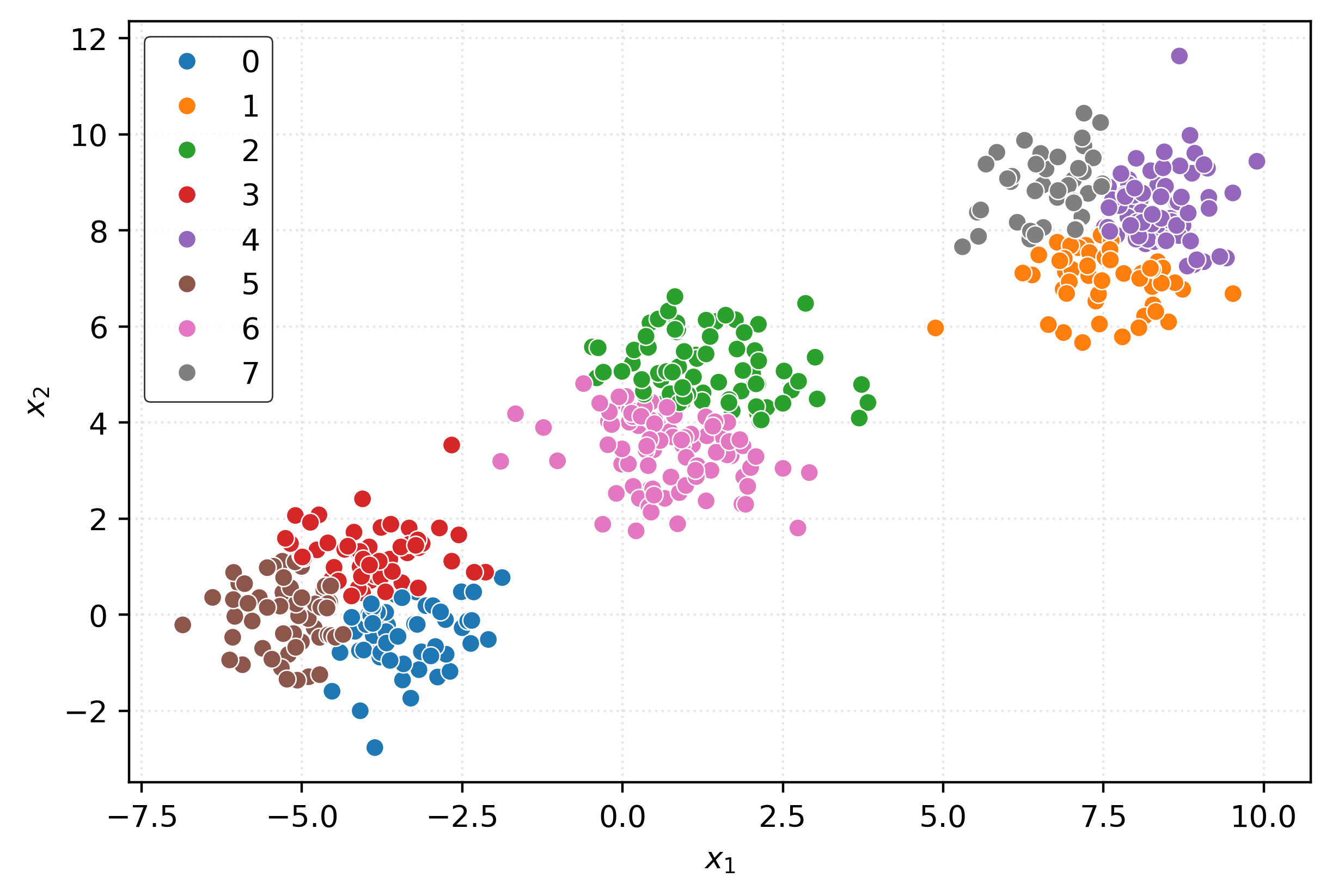
km3 = KMeans(n_clusters=3)
km3.fit(X)
clusters = km3.predict(X)
clusters
array([2, 1, 2, 1, 2, 0, 2, 2, 2, 2, 1, 2, 2, 0, 2, 2, 2, 2, 0, 0, 1, 1,
2, 2, 0, 2, 0, 1, 0, 1, 1, 2, 1, 1, 1, 1, 1, 2, 0, 0, 0, 0, 0, 2,
1, 1, 1, 0, 2, 1, 2, 2, 2, 2, 1, 2, 2, 1, 2, 1, 2, 2, 0, 2, 1, 0,
0, 0, 1, 0, 1, 1, 2, 2, 1, 1, 2, 1, 1, 1, 2, 0, 1, 2, 0, 1, 1, 1,
2, 1, 0, 2, 2, 0, 2, 1, 0, 1, 1, 2, 2, 2, 1, 1, 2, 2, 0, 2, 2, 1,
1, 2, 1, 0, 0, 0, 0, 0, 1, 2, 0, 0, 0, 0, 2, 0, 0, 0, 1, 2, 0, 2,
2, 2, 0, 1, 0, 0, 1, 0, 2, 0, 2, 0, 2, 0, 1, 0, 2, 1, 2, 0, 1, 1,
0, 2, 2, 1, 2, 0, 1, 2, 1, 0, 1, 1, 1, 0, 0, 1, 0, 1, 0, 2, 1, 0,
2, 2, 0, 1, 0, 2, 1, 0, 1, 2, 1, 1, 0, 2, 0, 1, 2, 0, 2, 0, 2, 1,
1, 2, 0, 0, 0, 0, 2, 0, 0, 0, 1, 1, 0, 0, 0, 0, 1, 0, 2, 1, 0, 1,
0, 1, 0, 1, 1, 2, 0, 1, 2, 1, 2, 2, 1, 1, 1, 0, 2, 0, 2, 1, 1, 1,
2, 0, 2, 0, 2, 0, 0, 0, 2, 2, 2, 1, 2, 0, 1, 2, 0, 1, 2, 2, 2, 0,
0, 2, 1, 1, 1, 2, 1, 2, 0, 2, 0, 1, 2, 2, 2, 2, 1, 0, 2, 2, 1, 0,
2, 1, 1, 0, 1, 2, 2, 2, 1, 2, 1, 1, 2, 0, 1, 2, 1, 0, 2, 0, 1, 2,
1, 0, 0, 1, 2, 0, 2, 0, 0, 1, 0, 2, 1, 1, 1, 1, 0, 0, 1, 2, 0, 1,
2, 0, 2, 2, 1, 1, 0, 1, 1, 1, 0, 0, 2, 0, 0, 1, 2, 2, 1, 1, 1, 0,
1, 0, 2, 1, 1, 0, 0, 0, 1, 2, 0, 0, 2, 0, 2, 0, 0, 0, 0, 2, 1, 2,
1, 0, 0, 2, 2, 1, 2, 1, 0, 1, 2, 0, 0, 2, 2, 2, 1, 0, 2, 0, 0, 0,
2, 1, 2, 2, 2, 0, 1, 1, 2, 1, 1, 0, 2, 0, 2, 0, 2, 1, 1, 2, 2, 2,
1, 1, 2, 2, 0, 0, 2, 0, 1, 0, 2, 0, 1, 0, 2, 1, 1, 0, 1, 2, 1, 1,
0, 0, 0, 1, 0, 1, 1, 1, 2, 2, 2, 0, 1, 1, 0, 1, 0, 0, 1, 0, 1, 2,
2, 1, 0, 2, 0, 0, 2, 0, 2, 0, 2, 2, 2, 1, 1, 0, 1, 2, 1, 1, 0, 1,
0, 1, 1, 0, 2, 1, 2, 0, 1, 2, 0, 2, 0, 1, 0, 0], dtype=int32)fig, ax = plt.subplots(figsize=(6, 4))
sns.scatterplot(
x=X[:, 0],
y=X[:, 1],
hue=pd.Categorical(clusters),
ax=ax,
)
plt.xlabel(r"$x_1$")
plt.ylabel(r"$x_2$")
plt.show()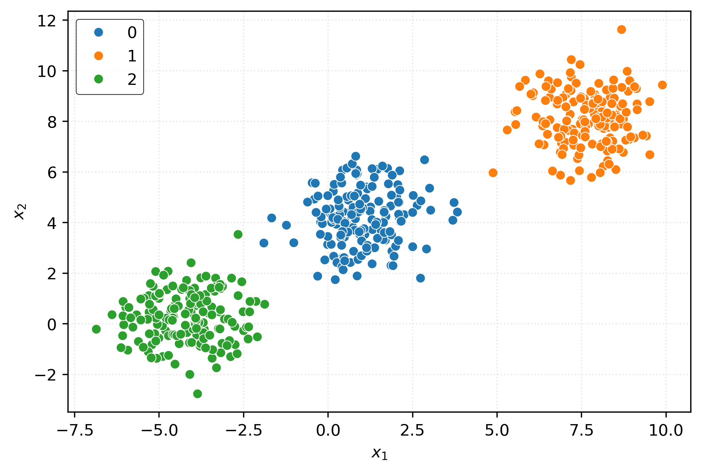
# check center of each learned cluster
km3.cluster_centers_
array([[ 7.672 , 8.1113],
[ 1.0145, 4.2032],
[-4.1873, 0.2754]])# check cost
km3.inertia_1005.8251148922151cost = []
for k in range(1, 11):
kmeans = KMeans(n_clusters=k, random_state=0)
kmeans.fit(X)
cost.append(kmeans.inertia_)fig, ax = plt.subplots(figsize=(6, 4))
ax.plot(range(1, 11), cost, marker="o")
ax.set_title("Elbow Plot")
ax.set_xlabel("Number of Clusters (k)")
ax.set_ylabel("Cost (Within Cluster Sum of Squares)")
plt.show()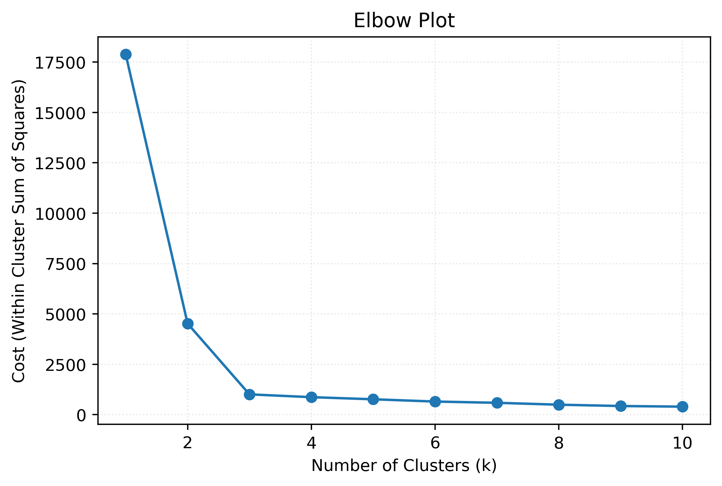
Additional Clustering Methods
X, _ = make_blobs(
    n_samples=500,
    n_features=2,
    cluster_std=1,
    random_state=3,
)
DBSCAN
dbscan = DBSCAN()
clusters = dbscan.fit_predict(X)
clusters
array([ 0, 1, 0, -1, 0, 2, 0, 0, 0, 0, 1, 0, 0, 2, 0, 0, 0,
0, -1, 2, 1, 1, 0, 0, 2, 0, 2, 1, 2, 1, -1, 0, 1, 1,
-1, 1, 1, 0, 2, 2, 2, 2, 2, 0, 1, 1, 1, 2, 0, 1, 0,
0, 0, 0, 1, 3, -1, 1, 0, 1, 0, 0, 2, 0, 1, 2, 2, -1,
1, 2, 1, 1, 0, 0, -1, -1, 0, 1, 1, 1, 0, -1, 1, 0, -1,
1, -1, 1, 0, 1, 2, 0, 3, 2, 0, 1, 2, 1, 1, 0, 0, -1,
1, 1, 0, 0, 2, 0, 0, 1, 1, 0, 1, 2, 2, 2, 2, 2, 1,
3, 2, 2, 2, 2, 0, 2, 2, 2, 1, 0, 2, 0, 0, 0, 2, 1,
2, 2, 1, 2, 0, 2, 0, 2, 0, 2, -1, 2, 0, -1, 0, 2, 1,
1, 2, 0, 0, 1, 0, 2, 1, 0, 1, 2, 1, 1, 1, 2, 2, 1,
-1, 1, 2, 0, 1, 2, 3, 0, 2, 1, 2, 0, 1, 2, 1, 0, 1,
1, 2, 0, 2, 1, -1, -1, 0, 2, 0, 1, 1, 0, 2, 2, 2, 2,
0, 2, 2, -1, 1, 1, 2, 2, 2, 2, 1, 2, 3, 1, -1, 1, 2,
1, 2, 1, 1, 0, 2, 1, 0, 1, -1, 0, 1, 1, 1, 2, 0, 2,
0, 1, 1, 1, 0, 2, 0, 2, 0, -1, 2, 2, 0, 0, 0, 1, 0,
2, 1, 0, 2, 1, 0, 0, 0, 2, 2, 0, 1, 1, -1, 0, 1, 0,
2, 0, 2, -1, 0, 0, 0, 0, 1, 2, 0, 0, 1, 2, -1, 1, 1,
2, 1, 0, 0, 0, 1, 0, 1, 1, 0, 2, 1, 0, 1, 2, 0, 2,
1, 0, 1, 2, 2, 1, 0, -1, 0, 2, 2, 1, 2, -1, 1, 1, 1,
1, 2, 2, 1, 0, 2, -1, 0, 2, 0, 0, 1, 1, 2, 1, 1, 1,
2, 2, 0, 2, 2, 1, 0, 0, 1, 1, 1, 2, 1, 2, 0, 1, 1,
2, 2, 2, 1, 0, 2, 2, 0, 2, -1, 2, 2, 2, 2, 0, 1, 0,
1, 2, 2, 0, 0, 1, 0, 1, 2, 1, 0, 2, 2, 0, 0, 0, 1,
2, 0, 2, 2, 2, 0, 1, 0, 0, 0, 2, 1, 1, 0, 1, 1, 2,
0, 2, 0, 2, -1, 1, 1, 0, 0, 0, 1, 1, 0, 0, 2, -1, 0,
2, 1, 2, 0, 2, 1, 2, -1, 1, 1, 2, 1, 0, -1, 1, 2, 2,
2, 1, 2, 1, 1, 1, 0, 0, 0, 2, 1, 1, 2, -1, 2, 2, 1,
2, 1, 0, 0, 1, 2, 0, 2, 2, 0, -1, 0, 2, 0, 0, 0, 1,
1, 2, 1, 0, 1, 1, 2, 1, 2, 1, 1, 2, 0, 1, 3, 2, -1,
0, 2, 0, -1, 1, -1, 2])fig, ax = plt.subplots(figsize=(6, 4))
sns.scatterplot(
x=X[:, 0],
y=X[:, 1],
hue=pd.Categorical(clusters),
ax=ax,
)
plt.xlabel(r"$x_1$")
plt.ylabel(r"$x_2$")
plt.show()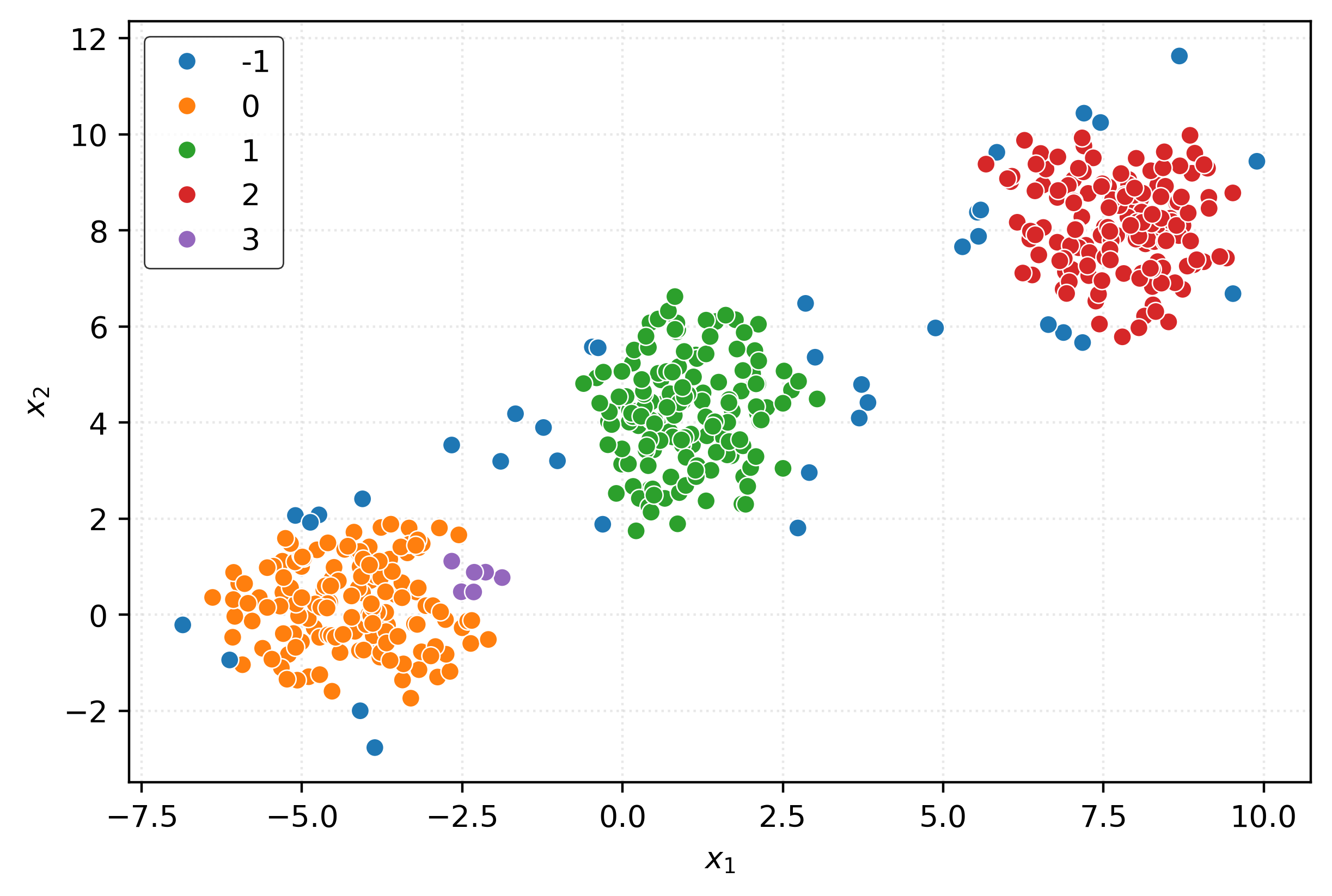
dbscan = DBSCAN(min_samples=25, eps=1.5)
clusters = dbscan.fit_predict(X)
clusters
array([ 0, 1, 0, 1, 0, 2, 0, 0, 0, 0, 1, 0, 0, 2, 0, 0, 0,
0, 2, 2, 1, 1, 0, 0, 2, 0, 2, 1, 2, 1, 1, 0, 1, 1,
1, 1, 1, 0, 2, 2, 2, 2, 2, 0, 1, 1, 1, 2, 0, 1, 0,
0, 0, 0, 1, 0, 0, 1, 0, 1, 0, 0, 2, 0, 1, 2, 2, 2,
1, 2, 1, 1, 0, 0, 1, -1, 0, 1, 1, 1, 0, -1, 1, 0, 2,
1, 1, 1, 0, 1, 2, 0, 0, 2, 0, 1, 2, 1, 1, 0, 0, -1,
1, 1, 0, 0, 2, 0, 0, 1, 1, 0, 1, 2, 2, 2, 2, 2, 1,
0, 2, 2, 2, 2, 0, 2, 2, 2, 1, 0, 2, 0, 0, 0, 2, 1,
2, 2, 1, 2, 0, 2, 0, 2, 0, 2, 1, 2, 0, 1, 0, 2, 1,
1, 2, 0, 0, 1, 0, 2, 1, 0, 1, 2, 1, 1, 1, 2, 2, 1,
2, 1, 2, 0, 1, 2, 0, 0, 2, 1, 2, 0, 1, 2, 1, 0, 1,
1, 2, 0, 2, 1, 0, 2, 0, 2, 0, 1, 1, 0, 2, 2, 2, 2,
0, 2, 2, -1, 1, 1, 2, 2, 2, 2, 1, 2, 0, 1, 2, 1, 2,
1, 2, 1, 1, 0, 2, 1, 0, 1, 0, 0, 1, 1, 1, 2, 0, 2,
0, 1, 1, 1, 0, 2, 0, 2, 0, 2, 2, 2, 0, 0, 0, 1, 0,
2, 1, 0, 2, 1, 0, 0, 0, 2, 2, 0, 1, 1, 1, 0, 1, 0,
2, 0, 2, 1, 0, 0, 0, 0, 1, 2, 0, 0, 1, 2, 0, 1, 1,
2, 1, 0, 0, 0, 1, 0, 1, 1, 0, 2, 1, 0, 1, 2, 0, 2,
1, 0, 1, 2, 2, 1, 0, 2, 0, 2, 2, 1, 2, 0, 1, 1, 1,
1, 2, 2, 1, 0, 2, 1, 0, 2, 0, 0, 1, 1, 2, 1, 1, 1,
2, 2, 0, 2, 2, 1, 0, 0, 1, 1, 1, 2, 1, 2, 0, 1, 1,
2, 2, 2, 1, 0, 2, 2, 0, 2, 0, 2, 2, 2, 2, 0, 1, 0,
1, 2, 2, 0, 0, 1, 0, 1, 2, 1, 0, 2, 2, 0, 0, 0, 1,
2, 0, 2, 2, 2, 0, 1, 0, 0, 0, 2, 1, 1, 0, 1, 1, 2,
0, 2, 0, 2, 0, 1, 1, 0, 0, 0, 1, 1, 0, 0, 2, 2, 0,
2, 1, 2, 0, 2, 1, 2, 0, 1, 1, 2, 1, 0, 1, 1, 2, 2,
2, 1, 2, 1, 1, 1, 0, 0, 0, 2, 1, 1, 2, 1, 2, 2, 1,
2, 1, 0, 0, 1, 2, 0, 2, 2, 0, 2, 0, 2, 0, 0, 0, 1,
1, 2, 1, 0, 1, 1, 2, 1, 2, 1, 1, 2, 0, 1, 0, 2, 1,
0, 2, 0, 2, 1, 2, 2])fig, ax = plt.subplots(figsize=(6, 4))
sns.scatterplot(
x=X[:, 0],
y=X[:, 1],
hue=pd.Categorical(clusters),
ax=ax,
)
plt.xlabel(r"$x_1$")
plt.ylabel(r"$x_2$")
plt.show()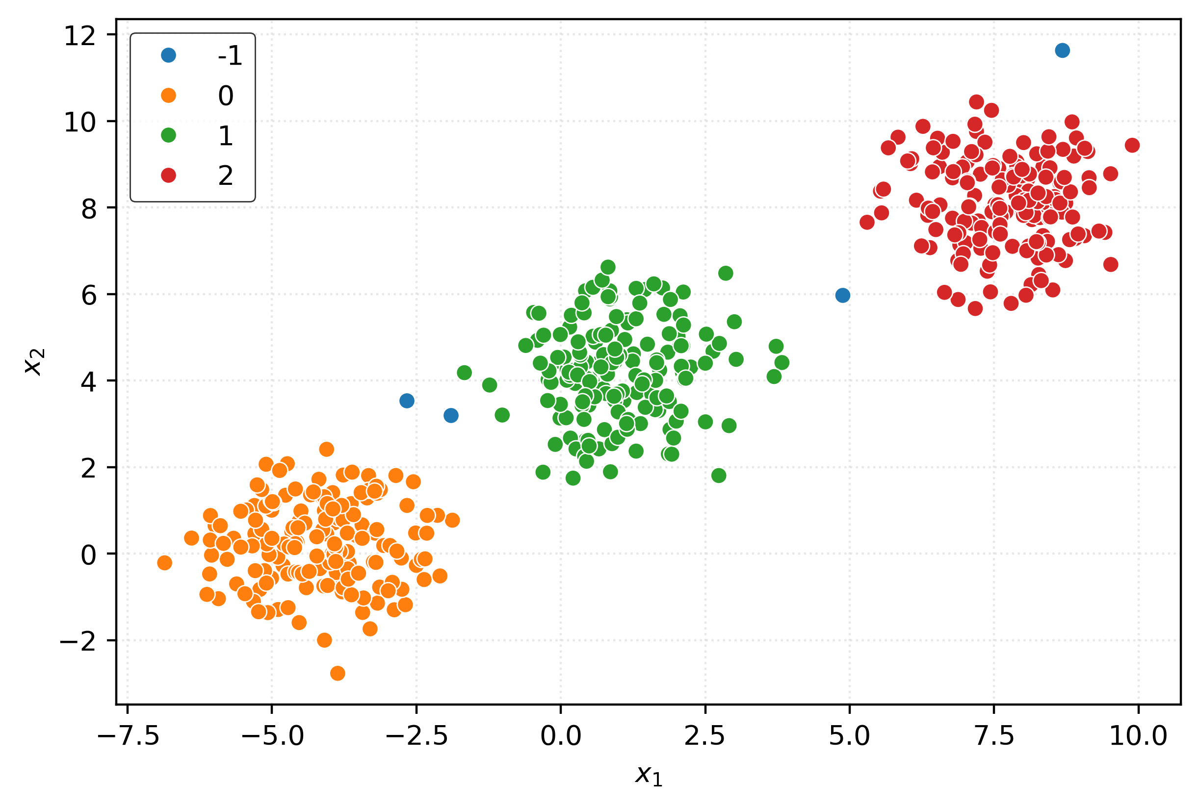
Agglomerative Clustering
ac = AgglomerativeClustering()
clusters = ac.fit_predict(X)
clusters
array([0, 0, 0, 0, 0, 1, 0, 0, 0, 0, 0, 0, 0, 1, 0, 0, 0, 0, 1, 1, 0, 0,
0, 0, 1, 0, 1, 0, 1, 0, 0, 0, 0, 0, 0, 0, 0, 0, 1, 1, 1, 1, 1, 0,
0, 0, 0, 1, 0, 0, 0, 0, 0, 0, 0, 0, 0, 0, 0, 0, 0, 0, 1, 0, 0, 1,
1, 1, 0, 1, 0, 0, 0, 0, 0, 0, 0, 0, 0, 0, 0, 1, 0, 0, 1, 0, 0, 0,
0, 0, 1, 0, 0, 1, 0, 0, 1, 0, 0, 0, 0, 0, 0, 0, 0, 0, 1, 0, 0, 0,
0, 0, 0, 1, 1, 1, 1, 1, 0, 0, 1, 1, 1, 1, 0, 1, 1, 1, 0, 0, 1, 0,
0, 0, 1, 0, 1, 1, 0, 1, 0, 1, 0, 1, 0, 1, 0, 1, 0, 0, 0, 1, 0, 0,
1, 0, 0, 0, 0, 1, 0, 0, 0, 1, 0, 0, 0, 1, 1, 0, 1, 0, 1, 0, 0, 1,
0, 0, 1, 0, 1, 0, 0, 1, 0, 0, 0, 0, 1, 0, 1, 0, 0, 1, 0, 1, 0, 0,
0, 0, 1, 1, 1, 1, 0, 1, 1, 0, 0, 0, 1, 1, 1, 1, 0, 1, 0, 0, 1, 0,
1, 0, 1, 0, 0, 0, 1, 0, 0, 0, 0, 0, 0, 0, 0, 1, 0, 1, 0, 0, 0, 0,
0, 1, 0, 1, 0, 1, 1, 1, 0, 0, 0, 0, 0, 1, 0, 0, 1, 0, 0, 0, 0, 1,
1, 0, 0, 0, 0, 0, 0, 0, 1, 0, 1, 0, 0, 0, 0, 0, 0, 1, 0, 0, 0, 1,
0, 0, 0, 1, 0, 0, 0, 0, 0, 0, 0, 0, 0, 1, 0, 0, 0, 1, 0, 1, 0, 0,
0, 1, 1, 0, 0, 1, 0, 1, 1, 0, 1, 0, 0, 0, 0, 0, 1, 1, 0, 0, 1, 0,
0, 1, 0, 0, 0, 0, 1, 0, 0, 0, 1, 1, 0, 1, 1, 0, 0, 0, 0, 0, 0, 1,
0, 1, 0, 0, 0, 1, 1, 1, 0, 0, 1, 1, 0, 1, 0, 1, 1, 1, 1, 0, 0, 0,
0, 1, 1, 0, 0, 0, 0, 0, 1, 0, 0, 1, 1, 0, 0, 0, 0, 1, 0, 1, 1, 1,
0, 0, 0, 0, 0, 1, 0, 0, 0, 0, 0, 1, 0, 1, 0, 1, 0, 0, 0, 0, 0, 0,
0, 0, 0, 0, 1, 1, 0, 1, 0, 1, 0, 1, 0, 1, 0, 0, 0, 1, 0, 0, 0, 0,
1, 1, 1, 0, 1, 0, 0, 0, 0, 0, 0, 1, 0, 0, 1, 0, 1, 1, 0, 1, 0, 0,
0, 0, 1, 0, 1, 1, 0, 1, 0, 1, 0, 0, 0, 0, 0, 1, 0, 0, 0, 0, 1, 0,
1, 0, 0, 1, 0, 0, 0, 1, 0, 0, 1, 0, 1, 0, 1, 1])fig, ax = plt.subplots(figsize=(6, 4))
sns.scatterplot(
x=X[:, 0],
y=X[:, 1],
hue=pd.Categorical(clusters),
ax=ax,
)
plt.xlabel(r"$x_1$")
plt.ylabel(r"$x_2$")
plt.show()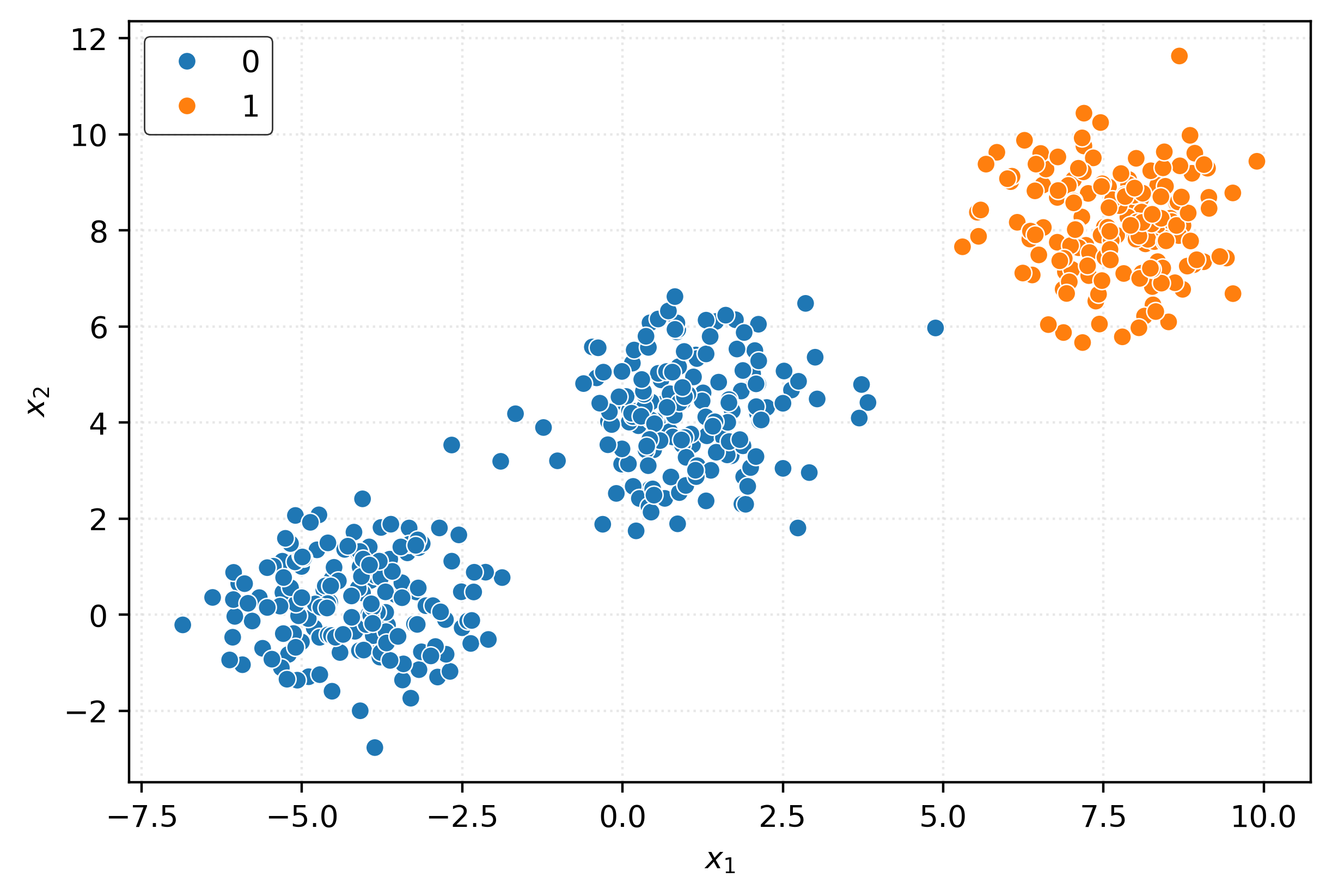
ac = AgglomerativeClustering(n_clusters=3)
clusters = ac.fit_predict(X)
clusters
array([1, 2, 1, 2, 1, 0, 1, 1, 1, 1, 2, 1, 1, 0, 1, 1, 1, 1, 0, 0, 2, 2,
1, 1, 0, 1, 0, 2, 0, 2, 2, 1, 2, 2, 2, 2, 2, 1, 0, 0, 0, 0, 0, 1,
2, 2, 2, 0, 1, 2, 1, 1, 1, 1, 2, 1, 1, 2, 1, 2, 1, 1, 0, 1, 2, 0,
0, 0, 2, 0, 2, 2, 1, 1, 2, 2, 1, 2, 2, 2, 1, 0, 2, 1, 0, 2, 2, 2,
1, 2, 0, 1, 1, 0, 1, 2, 0, 2, 2, 1, 1, 2, 2, 2, 1, 1, 0, 1, 1, 2,
2, 1, 2, 0, 0, 0, 0, 0, 2, 1, 0, 0, 0, 0, 1, 0, 0, 0, 2, 1, 0, 1,
1, 1, 0, 2, 0, 0, 2, 0, 1, 0, 1, 0, 1, 0, 2, 0, 1, 2, 1, 0, 2, 2,
0, 1, 1, 2, 1, 0, 2, 1, 2, 0, 2, 2, 2, 0, 0, 2, 0, 2, 0, 1, 2, 0,
1, 1, 0, 2, 0, 1, 2, 0, 2, 1, 2, 2, 0, 1, 0, 2, 1, 0, 1, 0, 1, 2,
2, 1, 0, 0, 0, 0, 1, 0, 0, 2, 2, 2, 0, 0, 0, 0, 2, 0, 1, 2, 0, 2,
0, 2, 0, 2, 2, 1, 0, 2, 1, 2, 1, 1, 2, 2, 2, 0, 1, 0, 1, 2, 2, 2,
1, 0, 1, 0, 1, 0, 0, 0, 1, 1, 1, 2, 1, 0, 2, 1, 0, 2, 1, 1, 1, 0,
0, 1, 2, 2, 2, 1, 2, 1, 0, 1, 0, 2, 1, 1, 1, 1, 2, 0, 1, 1, 2, 0,
1, 2, 2, 0, 2, 1, 1, 1, 2, 1, 2, 2, 1, 0, 2, 1, 2, 0, 1, 0, 2, 1,
2, 0, 0, 2, 1, 0, 1, 0, 0, 2, 0, 1, 2, 2, 2, 2, 0, 0, 2, 1, 0, 2,
1, 0, 1, 1, 2, 2, 0, 2, 2, 2, 0, 0, 1, 0, 0, 2, 1, 1, 2, 2, 2, 0,
2, 0, 1, 2, 2, 0, 0, 0, 2, 1, 0, 0, 1, 0, 1, 0, 0, 0, 0, 1, 2, 1,
2, 0, 0, 1, 1, 2, 1, 2, 0, 2, 1, 0, 0, 1, 1, 1, 2, 0, 1, 0, 0, 0,
1, 2, 1, 1, 1, 0, 2, 2, 1, 2, 2, 0, 1, 0, 1, 0, 1, 2, 2, 1, 1, 1,
2, 2, 1, 1, 0, 0, 1, 0, 2, 0, 1, 0, 2, 0, 1, 2, 2, 0, 2, 1, 2, 2,
0, 0, 0, 2, 0, 2, 2, 2, 1, 1, 1, 0, 2, 2, 0, 2, 0, 0, 2, 0, 2, 1,
1, 2, 0, 1, 0, 0, 1, 0, 1, 0, 1, 1, 1, 2, 2, 0, 2, 1, 2, 2, 0, 2,
0, 2, 2, 0, 1, 2, 1, 0, 2, 1, 0, 1, 0, 2, 0, 0])fig, ax = plt.subplots(figsize=(6, 4))
sns.scatterplot(
x=X[:, 0],
y=X[:, 1],
hue=pd.Categorical(clusters),
ax=ax,
)
plt.xlabel(r"$x_1$")
plt.ylabel(r"$x_2$")
plt.show()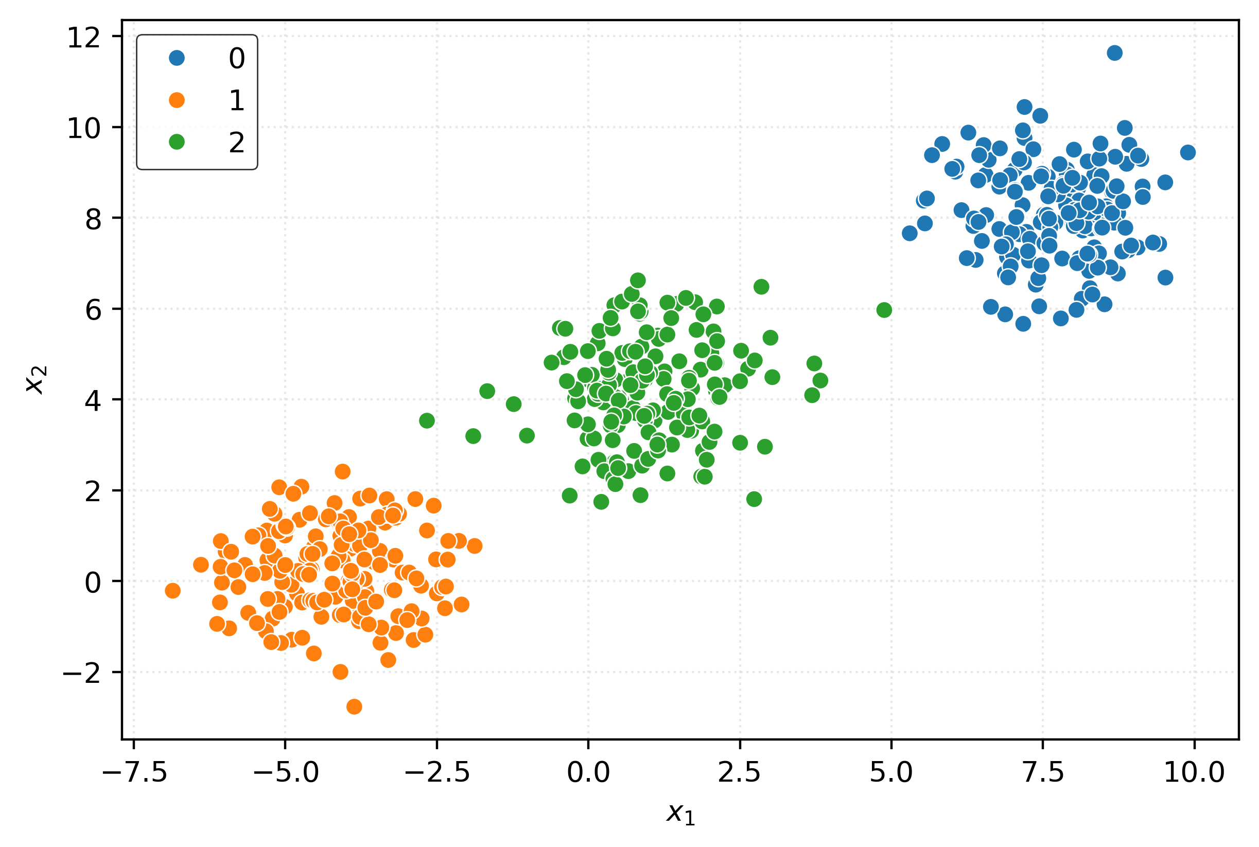
Density Estimation
Kernel Density Estimation
\[ f_h(x) = \frac{1}{nh} \sum_{i=1}^{n} K\left(\frac{x - x_i}{h}\right) \]
# generate a small sample
X = np.array([-2, -1.5, -1.3, -1, -0.5, 2, 5, 6]).reshape(-1, 1)

# fit KDE
kde = KernelDensity(bandwidth=1)
_ = kde.fit(X)

# get pdf values for the plot x values
x = np.linspace(X.min() - 3, X.max() + 3, 1000)
logprob = kde.score_samples(x.reshape(-1, 1))
pdf = np.exp(logprob)

# create rug plot
fig, ax = plt.subplots(figsize=(8, 4))
sns.rugplot(
    X.ravel(),
    color="dodgerblue",
    height=0.1,
    linewidth=2,
    expand_margins=False,
    zorder=2,
    ax=ax,
)

# add individual kernels
for x_i in X.ravel():
    kernel = norm.pdf(x, loc=x_i, scale=kde.bandwidth)
    ax.plot(
        x,
        kernel,
        color="lightblue",
        alpha=0.65,
        linestyle="--",
        zorder=1,
    )

# add the KDE
ax.plot(x, pdf, color="darkorange")
plt.show()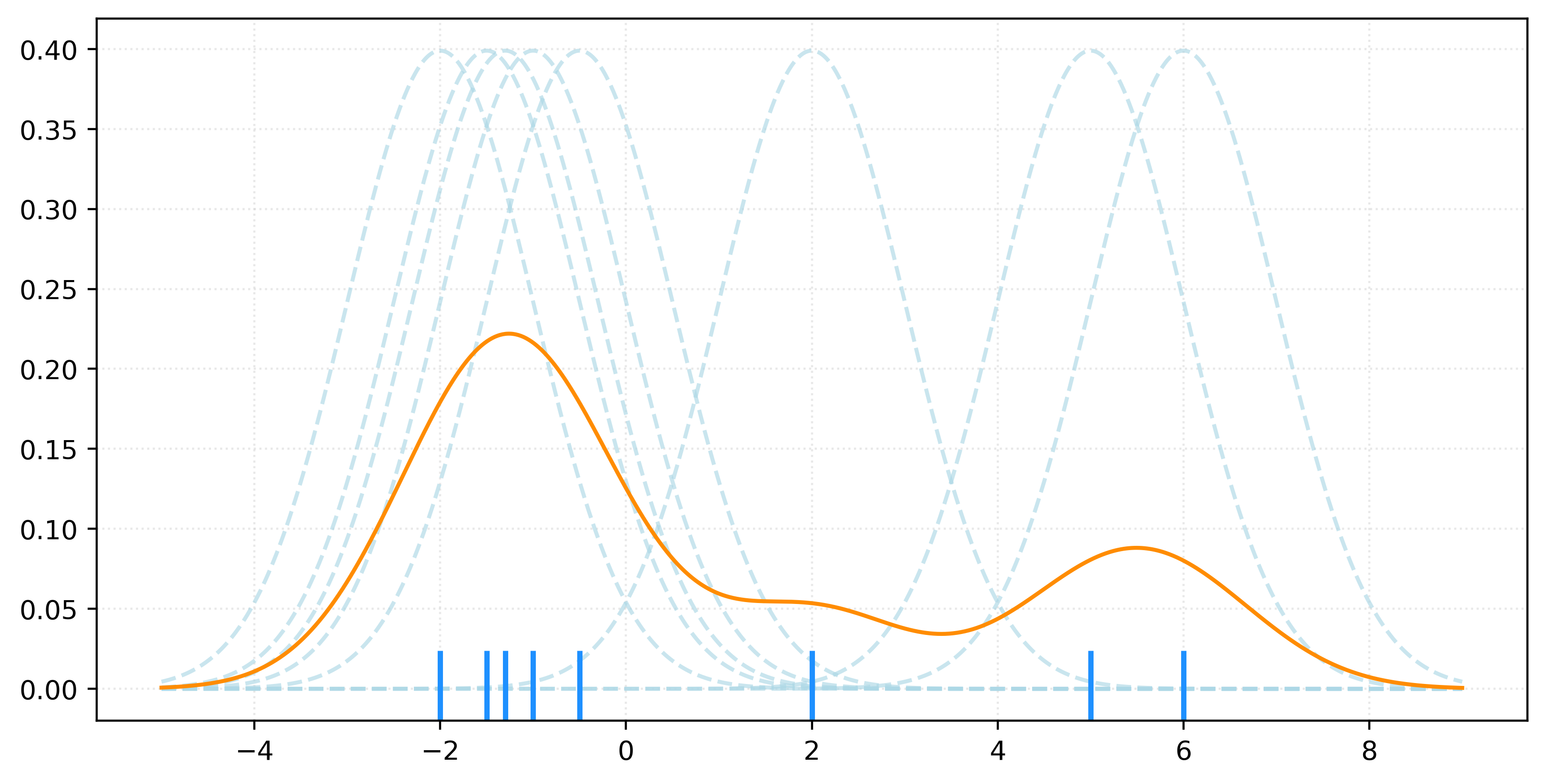
X, _ = make_blobs(
    n_samples=250,
    centers=2,
    n_features=1,
    cluster_std=[1.5, 3],
    random_state=42,
)
X[:10]
array([[-2.7877],
[ 6.0902],
[-1.6289],
[ 9.6637],
[-3.0007],
[-2.5015],
[-1.9457],
[10.6966],
[-1.9031],
[-3.5623]])fig, ax = plt.subplots()
sns.histplot(
X.ravel(),
bins=20,
stat="density",
color="lightgrey",
ax=ax,
)
sns.rugplot(
X.ravel(),
color="dodgerblue",
ax=ax,
)
plt.show()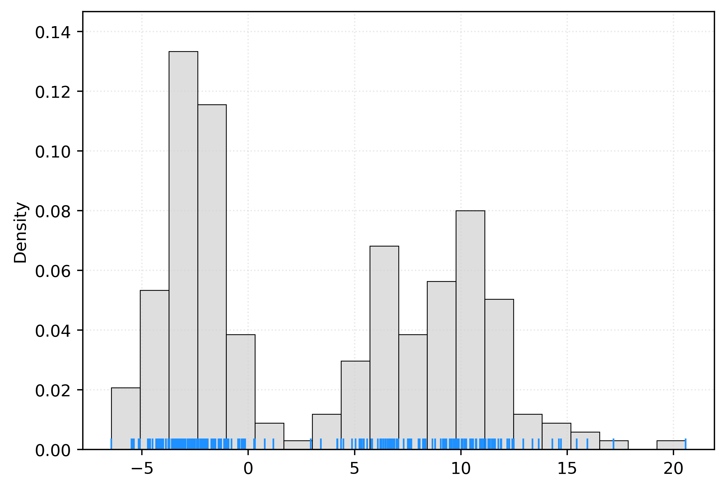
kde = KernelDensity(bandwidth=1)
_ = kde.fit(X)
# get pdf values for the plot x values
x = np.linspace(X.min(), X.max(), 1000)
logprob = kde.score_samples(x.reshape(-1, 1))
pdf = np.exp(logprob)
fig, ax = plt.subplots()
sns.histplot(
X.ravel(),
bins=20,
stat="density",
color="lightgrey",
ax=ax,
)
sns.rugplot(
X.ravel(),
color="dodgerblue",
ax=ax,
)
ax.plot(x, pdf, color="darkorange")
plt.show()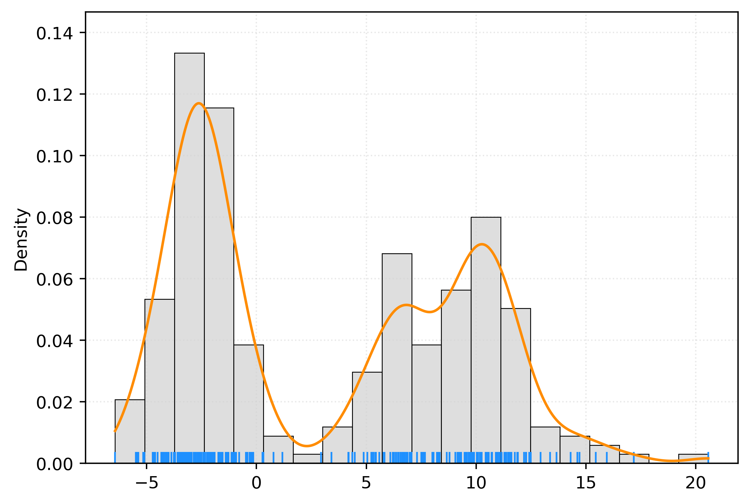
print(np.exp(kde.score_samples([[10]])))
print(np.mean(norm.pdf(10 - X.ravel())))
[0.0704]
0.07041697626037091# generate new samples from learned distribution
X_new = kde.sample(
n_samples=250,
random_state=42,
)fig, ax = plt.subplots()
sns.histplot(
X_new.ravel(),
bins=20,
stat="density",
color="lightgrey",
ax=ax,
)
sns.rugplot(
X.ravel(),
color="dodgerblue",
ax=ax,
)
plt.show()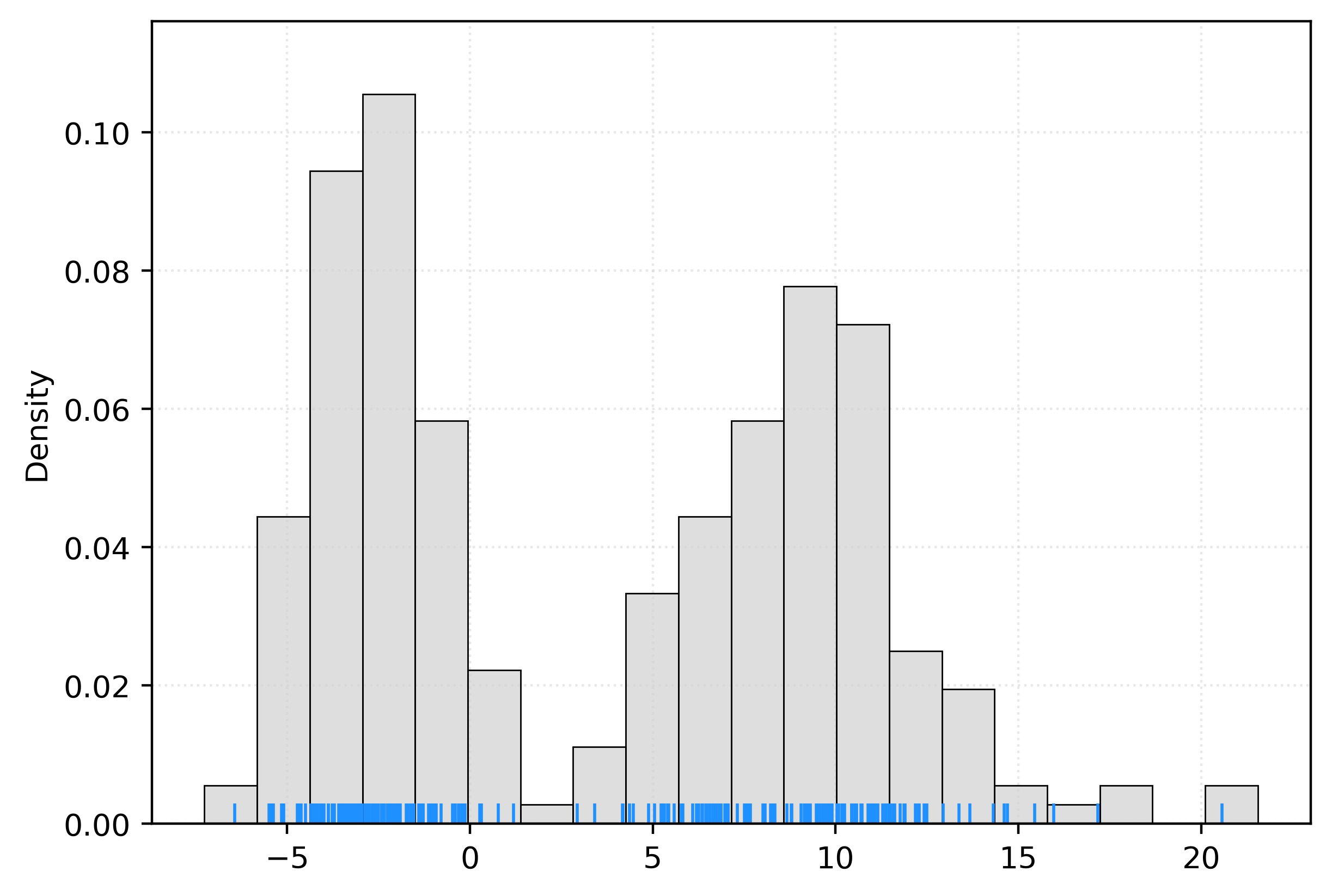
Gaussian Mixture Models
gmm = GaussianMixture(n_components=2)
gmm.fit(X)
gmm.predict(X)
array([0, 1, 0, 1, 0, 0, 0, 1, 0, 0, 0, 1, 0, 1, 1, 0, 0, 1, 1, 1, 0, 0,
0, 0, 1, 0, 0, 1, 1, 0, 1, 0, 0, 1, 1, 0, 0, 1, 0, 0, 1, 1, 0, 1,
0, 1, 1, 0, 0, 1, 0, 1, 0, 0, 0, 0, 0, 1, 1, 1, 1, 0, 0, 1, 1, 0,
0, 0, 0, 1, 0, 0, 1, 1, 0, 0, 0, 1, 1, 0, 1, 1, 0, 0, 0, 0, 1, 0,
0, 1, 1, 0, 1, 0, 1, 1, 1, 0, 1, 1, 0, 1, 0, 1, 0, 0, 1, 0, 1, 0,
1, 0, 1, 1, 0, 1, 1, 1, 0, 1, 1, 1, 0, 1, 0, 0, 0, 0, 1, 0, 0, 1,
1, 0, 1, 0, 1, 0, 1, 0, 0, 1, 1, 1, 0, 0, 1, 0, 1, 0, 0, 1, 1, 1,
0, 0, 1, 0, 0, 0, 1, 0, 0, 1, 1, 1, 1, 0, 0, 0, 0, 1, 0, 0, 1, 1,
1, 0, 0, 0, 1, 1, 0, 0, 0, 1, 1, 1, 1, 1, 1, 0, 1, 1, 1, 1, 0, 1,
1, 0, 0, 0, 1, 0, 1, 0, 0, 1, 1, 1, 1, 0, 1, 1, 0, 0, 0, 0, 0, 0,
0, 1, 1, 1, 1, 1, 1, 1, 0, 0, 1, 1, 1, 0, 1, 0, 1, 1, 1, 1, 0, 1,
0, 0, 0, 1, 1, 1, 1, 0])gmm.predict_proba(X[:10])array([[9.9981e-01, 1.9050e-04],
[1.7360e-08, 1.0000e+00],
[9.9897e-01, 1.0341e-03],
[6.6233e-17, 1.0000e+00],
[9.9985e-01, 1.4782e-04],
[9.9972e-01, 2.7546e-04],
[9.9938e-01, 6.1812e-04],
[9.5809e-20, 1.0000e+00],
[9.9934e-01, 6.6083e-04],
[9.9992e-01, 8.2492e-05]])gmm._estimate_log_prob(X[:10])array([[ -1.2687, -9.8468],
[-20.3862, -2.5295],
[ -1.513 , -8.3986],
[-39.2782, -2.0373],
[ -1.2973, -10.1291],
[ -1.2662, -9.4754],
[ -1.3791, -8.7797],
[-45.9369, -2.1574],
[ -1.3941, -8.7279],
[ -1.4823, -10.8974]])gmm.weights_array([0.4969, 0.5031])gmm.means_array([[-2.6271],
[ 9.1261]])gmm.covariances_array([[[1.9868]],
[[9.0691]]])np.sum(np.exp(gmm._estimate_log_prob(X[:10])) * gmm.weights_, axis=1)array([0.1398, 0.0401, 0.1096, 0.0656, 0.1358, 0.1401, 0.1252, 0.0582,
0.1233, 0.1129])np.exp(gmm.score_samples(X[:10]))array([0.1398, 0.0401, 0.1096, 0.0656, 0.1358, 0.1401, 0.1252, 0.0582,
0.1233, 0.1129])# get pdf values for the plot x values
x = np.linspace(X.min(), X.max(), 1000)
logprob = gmm.score_samples(x.reshape(-1, 1))
pdf = np.exp(logprob)
# create plot
fig, ax = plt.subplots()
sns.histplot(
X.ravel(),
bins=20,
stat="density",
color="lightgrey",
ax=ax,
)
sns.rugplot(
X.ravel(),
color="dodgerblue",
ax=ax,
)
ax.plot(x, pdf, color="darkorange")
plt.show()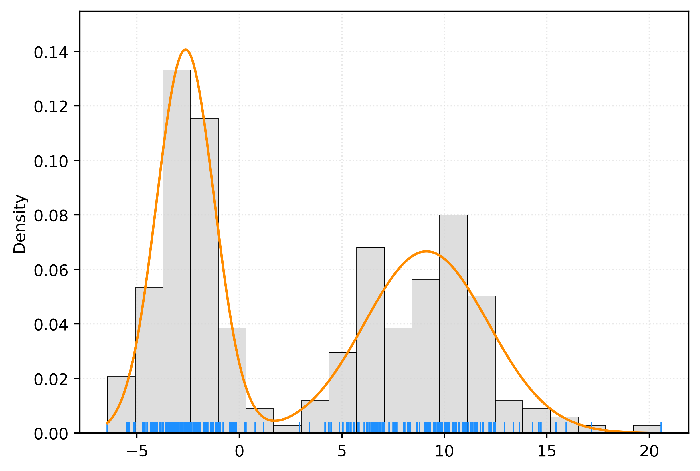
gmm.sample(n_samples=10)(array([[-4.1851],
[-1.5803],
[-5.9556],
[-2.4847],
[-2.6297],
[15.7682],
[ 7.7713],
[ 8.2724],
[ 7.0667],
[ 6.8943]]),
array([0, 0, 0, 0, 0, 1, 1, 1, 1, 1]))X, _ = make_blobs(
n_samples=500,
n_features=2,
cluster_std=[0.5, 2, 5],
random_state=3,
)
X.shape(500, 2)fig, ax = plt.subplots(figsize=(6, 4))
sns.scatterplot(
x=X[:, 0],
y=X[:, 1],
ax=ax,
)
plt.xlabel(r"$x_1$")
plt.ylabel(r"$x_2$")
plt.show()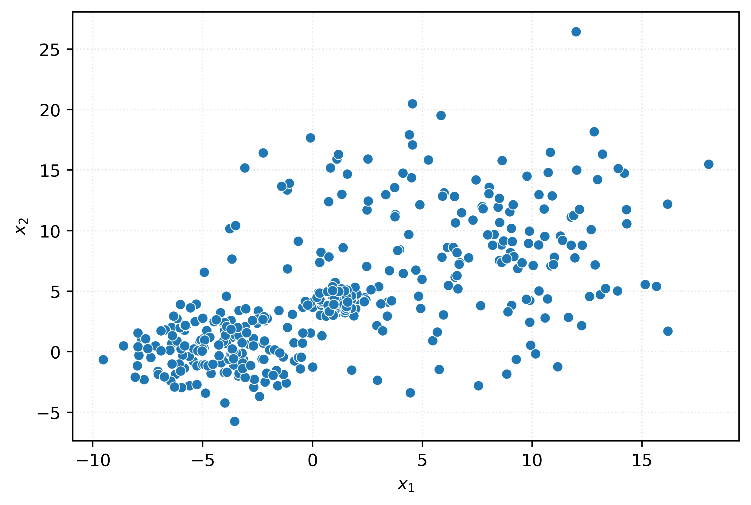
km3 = KMeans(n_clusters=3)
km3.fit(X)
clusters = km3.predict(X)
fig, ax = plt.subplots(figsize=(6, 4))
sns.scatterplot(
x=X[:, 0],
y=X[:, 1],
hue=pd.Categorical(clusters),
ax=ax,
)
plt.xlabel(r"$x_1$")
plt.ylabel(r"$x_2$")
plt.show()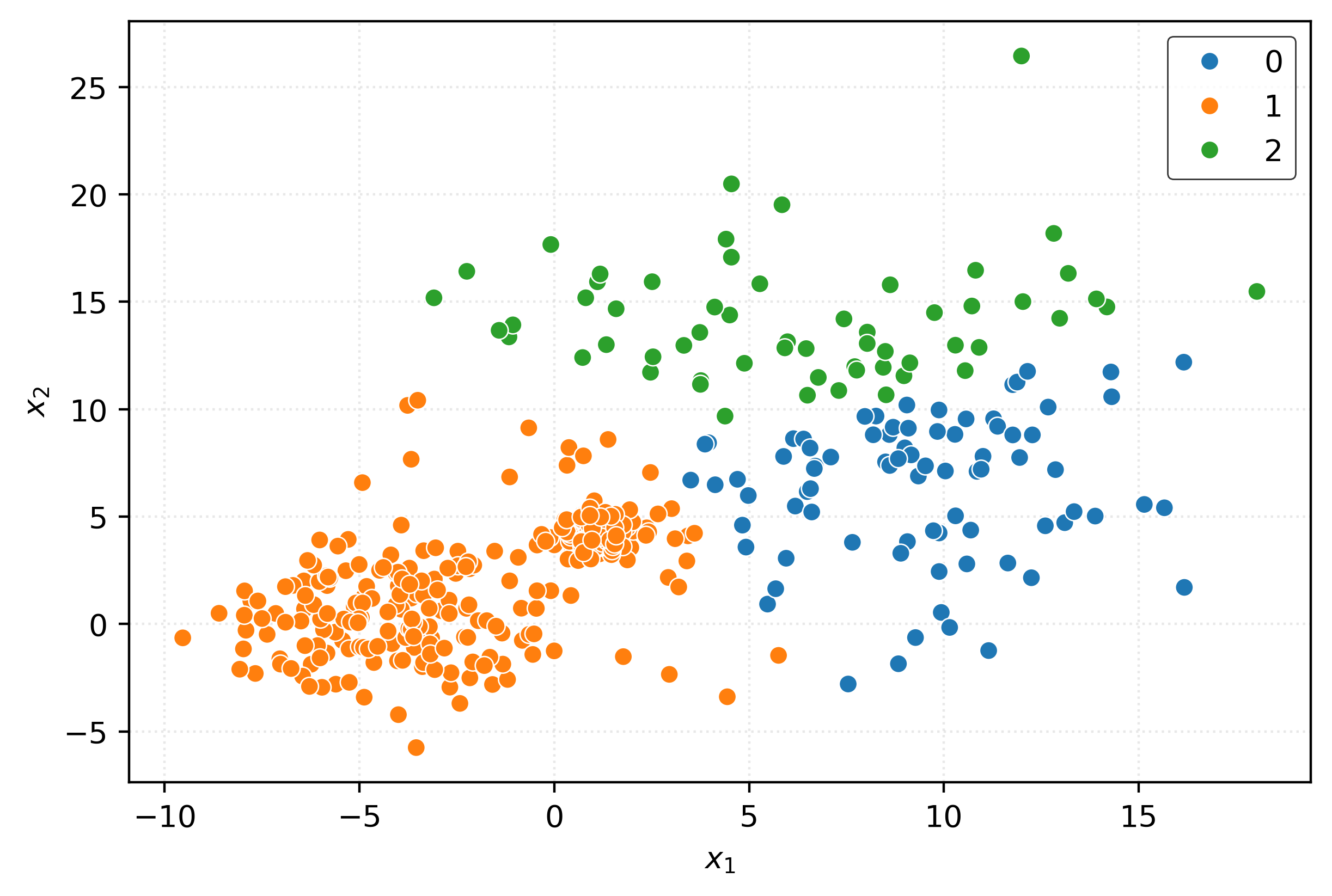
gmm = GaussianMixture(n_components=3)
gmm.fit(X)
clusters = gmm.predict(X)
fig, ax = plt.subplots(figsize=(6, 4))
sns.scatterplot(
x=X[:, 0],
y=X[:, 1],
hue=pd.Categorical(clusters),
ax=ax,
)
plt.xlabel(r"$x_1$")
plt.ylabel(r"$x_2$")
plt.show()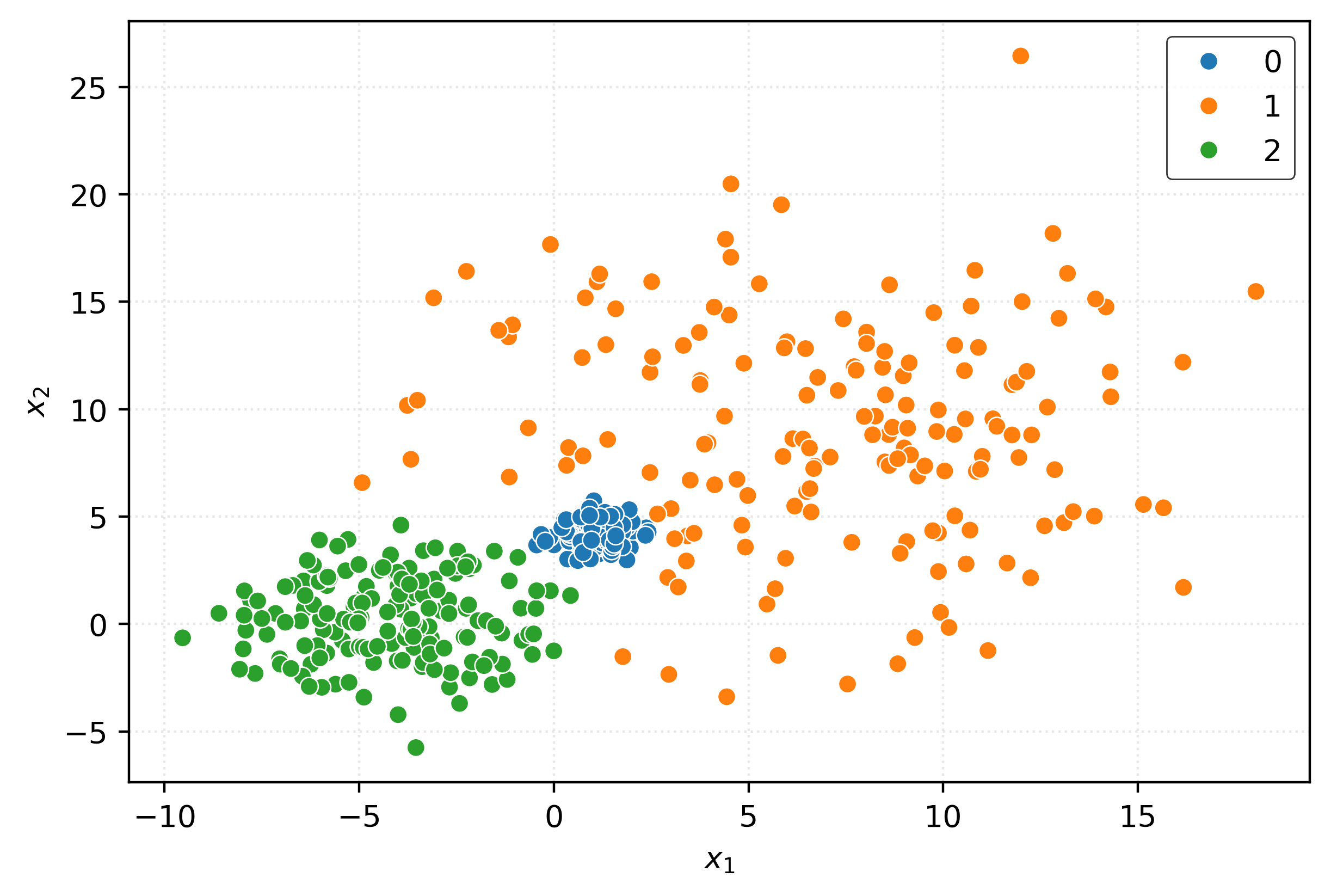
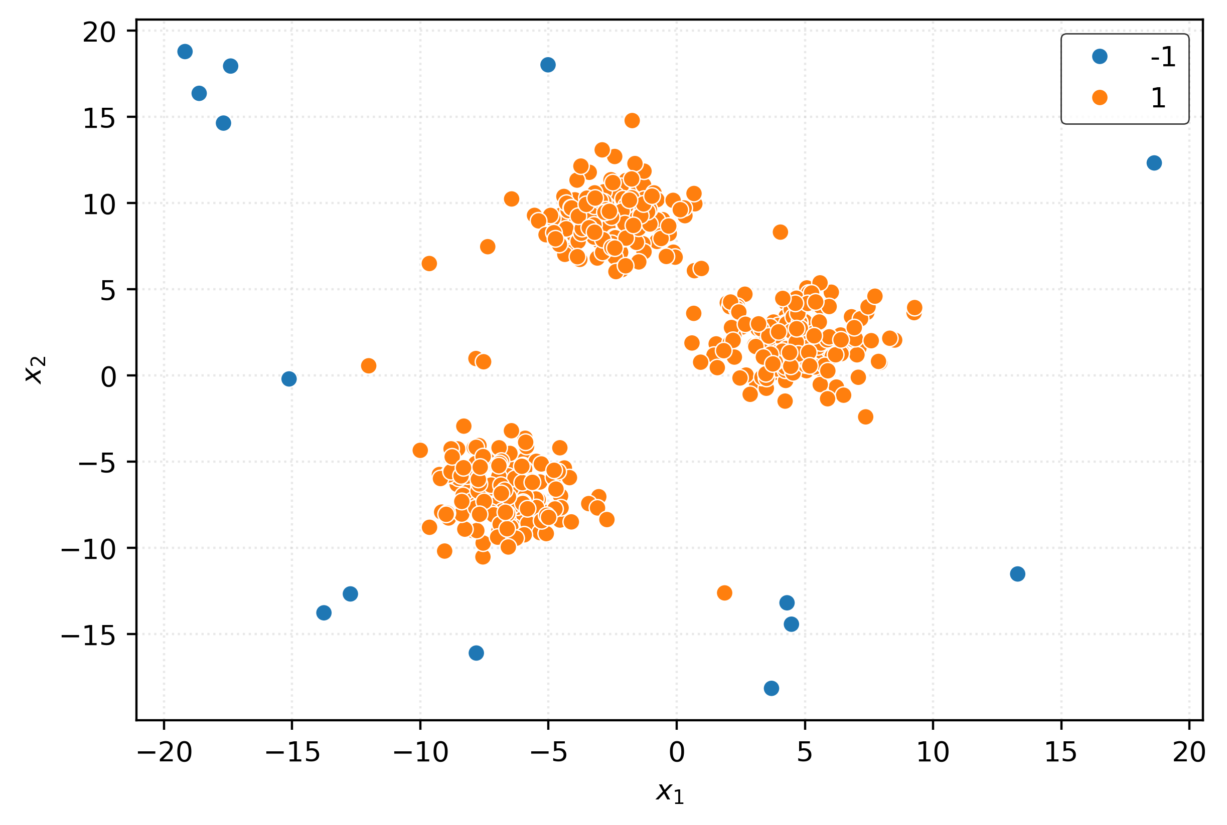
Outlier Detection
X, _ = make_blobs(
    n_samples=500,
    centers=3,
    n_features=2,
    cluster_std=1.5,
    random_state=42,
)
outliers = np.random.RandomState(42).uniform(
    low=-20,
    high=20,
    size=(25, 2),
)
X = np.vstack((X, outliers))
X
array([[ -5.1557, -7.9349],
[ 0.5945, 1.8917],
[ 7.9246, 0.7607],
...,
[ -9.6488, 6.5009],
[ -7.5316, 0.8027],
[ 1.8684, -12.6058]], shape=(525, 2))fig, ax = plt.subplots(figsize=(6, 4))
sns.scatterplot(
x=X[:, 0],
y=X[:, 1],
ax=ax,
)
plt.xlabel(r"$x_1$")
plt.ylabel(r"$x_2$")
plt.show()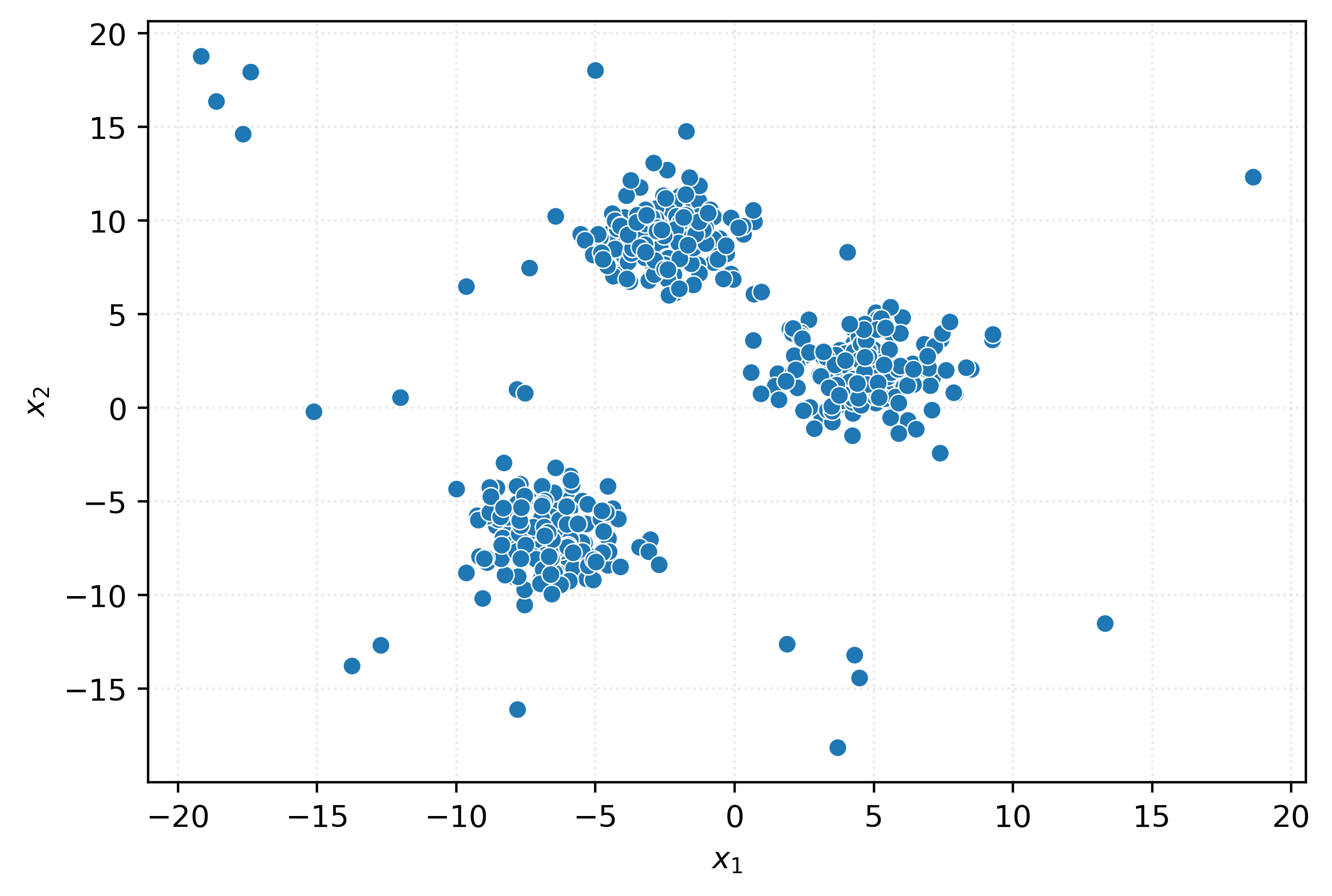
iso = IsolationForest(
    random_state=42,
)
_ = iso.fit(X)
inout = iso.predict(X)
inout
array([ 1, 1, -1, 1, 1, 1, -1, 1, 1, 1, 1, 1, 1, 1, 1, 1, 1,
1, 1, 1, 1, 1, 1, 1, 1, 1, 1, 1, 1, 1, 1, 1, 1, 1,
1, 1, 1, 1, 1, 1, 1, 1, 1, 1, 1, 1, 1, 1, 1, 1, -1,
1, 1, 1, 1, 1, 1, 1, 1, 1, 1, 1, 1, 1, 1, 1, 1, -1,
1, 1, 1, 1, 1, 1, 1, 1, 1, 1, 1, 1, 1, 1, 1, 1, 1,
1, 1, 1, 1, 1, 1, 1, 1, 1, 1, 1, -1, 1, 1, 1, 1, 1,
1, 1, 1, 1, 1, -1, 1, 1, 1, 1, 1, 1, 1, 1, 1, 1, 1,
1, 1, 1, 1, 1, 1, 1, 1, 1, 1, 1, 1, 1, 1, 1, 1, 1,
1, 1, 1, 1, 1, 1, 1, 1, 1, 1, 1, 1, 1, 1, 1, 1, 1,
1, 1, 1, 1, 1, 1, 1, 1, 1, 1, 1, 1, 1, 1, 1, 1, 1,
1, 1, 1, 1, 1, 1, 1, 1, 1, -1, 1, 1, 1, 1, 1, 1, 1,
1, 1, 1, 1, 1, 1, 1, 1, -1, 1, 1, 1, 1, 1, 1, 1, 1,
1, 1, 1, 1, 1, 1, 1, -1, 1, 1, 1, 1, 1, 1, 1, 1, 1,
1, 1, 1, 1, 1, 1, 1, 1, 1, 1, 1, 1, 1, 1, 1, -1, 1,
1, 1, 1, 1, 1, 1, 1, 1, 1, -1, 1, 1, 1, 1, 1, 1, -1,
1, 1, 1, 1, 1, -1, 1, 1, 1, 1, 1, 1, 1, 1, 1, 1, 1,
1, 1, 1, 1, 1, 1, 1, 1, 1, 1, 1, 1, 1, 1, 1, 1, 1,
1, 1, 1, 1, 1, 1, -1, 1, 1, 1, 1, 1, 1, 1, 1, 1, -1,
1, 1, 1, 1, 1, 1, -1, 1, 1, 1, 1, 1, 1, 1, 1, 1, 1,
1, 1, 1, -1, 1, 1, 1, 1, 1, 1, 1, 1, 1, 1, 1, 1, 1,
1, 1, 1, 1, 1, 1, 1, 1, 1, 1, 1, 1, 1, 1, 1, 1, 1,
1, 1, 1, 1, 1, 1, 1, 1, 1, 1, 1, 1, 1, 1, 1, 1, 1,
1, 1, 1, 1, 1, 1, 1, 1, 1, -1, 1, -1, 1, 1, 1, 1, 1,
1, 1, 1, 1, 1, 1, 1, 1, 1, -1, 1, 1, 1, 1, 1, 1, 1,
1, 1, 1, 1, 1, 1, 1, 1, 1, 1, 1, 1, 1, 1, 1, 1, 1,
1, 1, 1, 1, -1, -1, 1, -1, 1, 1, 1, 1, -1, 1, -1, 1, 1,
1, 1, 1, 1, 1, -1, 1, 1, 1, 1, 1, 1, 1, 1, 1, -1, 1,
1, 1, 1, 1, 1, 1, 1, 1, 1, 1, 1, 1, 1, -1, 1, 1, 1,
1, 1, 1, 1, 1, 1, -1, 1, 1, 1, 1, 1, -1, 1, 1, 1, 1,
1, 1, 1, 1, 1, 1, 1, -1, -1, -1, -1, -1, -1, -1, -1, -1, -1,
-1, 1, 1, -1, -1, -1, -1, -1, -1, -1, -1, -1, -1, -1, -1])fig, ax = plt.subplots(figsize=(6, 4))
sns.scatterplot(
x=X[:, 0],
y=X[:, 1],
hue=pd.Categorical(inout),
ax=ax,
)
plt.xlabel(r"$x_1$")
plt.ylabel(r"$x_2$")
plt.show()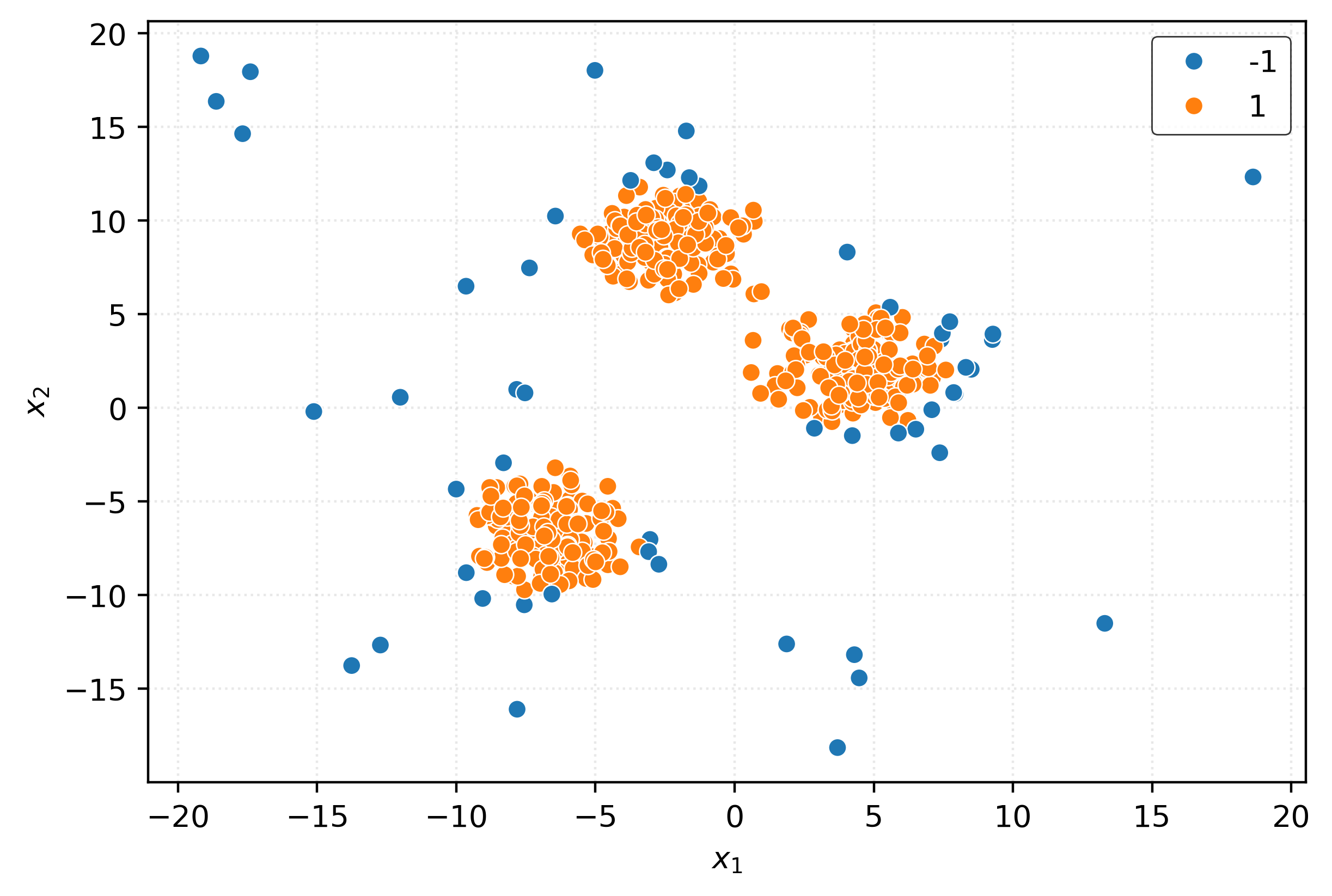
iso = IsolationForest(
    contamination=0.025,
    random_state=42,
)
_ = iso.fit(X)
inout = iso.predict(X)
inout
array([ 1, 1, 1, 1, 1, 1, 1, 1, 1, 1, 1, 1, 1, 1, 1, 1, 1,
1, 1, 1, 1, 1, 1, 1, 1, 1, 1, 1, 1, 1, 1, 1, 1, 1,
1, 1, 1, 1, 1, 1, 1, 1, 1, 1, 1, 1, 1, 1, 1, 1, 1,
1, 1, 1, 1, 1, 1, 1, 1, 1, 1, 1, 1, 1, 1, 1, 1, 1,
1, 1, 1, 1, 1, 1, 1, 1, 1, 1, 1, 1, 1, 1, 1, 1, 1,
1, 1, 1, 1, 1, 1, 1, 1, 1, 1, 1, 1, 1, 1, 1, 1, 1,
1, 1, 1, 1, 1, 1, 1, 1, 1, 1, 1, 1, 1, 1, 1, 1, 1,
1, 1, 1, 1, 1, 1, 1, 1, 1, 1, 1, 1, 1, 1, 1, 1, 1,
1, 1, 1, 1, 1, 1, 1, 1, 1, 1, 1, 1, 1, 1, 1, 1, 1,
1, 1, 1, 1, 1, 1, 1, 1, 1, 1, 1, 1, 1, 1, 1, 1, 1,
1, 1, 1, 1, 1, 1, 1, 1, 1, 1, 1, 1, 1, 1, 1, 1, 1,
1, 1, 1, 1, 1, 1, 1, 1, 1, 1, 1, 1, 1, 1, 1, 1, 1,
1, 1, 1, 1, 1, 1, 1, 1, 1, 1, 1, 1, 1, 1, 1, 1, 1,
1, 1, 1, 1, 1, 1, 1, 1, 1, 1, 1, 1, 1, 1, 1, 1, 1,
1, 1, 1, 1, 1, 1, 1, 1, 1, 1, 1, 1, 1, 1, 1, 1, 1,
1, 1, 1, 1, 1, 1, 1, 1, 1, 1, 1, 1, 1, 1, 1, 1, 1,
1, 1, 1, 1, 1, 1, 1, 1, 1, 1, 1, 1, 1, 1, 1, 1, 1,
1, 1, 1, 1, 1, 1, 1, 1, 1, 1, 1, 1, 1, 1, 1, 1, 1,
1, 1, 1, 1, 1, 1, 1, 1, 1, 1, 1, 1, 1, 1, 1, 1, 1,
1, 1, 1, 1, 1, 1, 1, 1, 1, 1, 1, 1, 1, 1, 1, 1, 1,
1, 1, 1, 1, 1, 1, 1, 1, 1, 1, 1, 1, 1, 1, 1, 1, 1,
1, 1, 1, 1, 1, 1, 1, 1, 1, 1, 1, 1, 1, 1, 1, 1, 1,
1, 1, 1, 1, 1, 1, 1, 1, 1, 1, 1, 1, 1, 1, 1, 1, 1,
1, 1, 1, 1, 1, 1, 1, 1, 1, 1, 1, 1, 1, 1, 1, 1, 1,
1, 1, 1, 1, 1, 1, 1, 1, 1, 1, 1, 1, 1, 1, 1, 1, 1,
1, 1, 1, 1, 1, 1, 1, 1, 1, 1, 1, 1, 1, 1, 1, 1, 1,
1, 1, 1, 1, 1, 1, 1, 1, 1, 1, 1, 1, 1, 1, 1, 1, 1,
1, 1, 1, 1, 1, 1, 1, 1, 1, 1, 1, 1, 1, 1, 1, 1, 1,
1, 1, 1, 1, 1, 1, 1, 1, 1, 1, 1, 1, 1, 1, 1, 1, 1,
1, 1, 1, 1, 1, 1, 1, -1, 1, -1, -1, 1, -1, -1, -1, 1, 1,
-1, 1, 1, 1, -1, -1, -1, -1, -1, 1, -1, -1, 1, 1, 1])fig, ax = plt.subplots(figsize=(6, 4))
sns.scatterplot(
x=X[:, 0],
y=X[:, 1],
hue=pd.Categorical(inout),
ax=ax,
)
plt.xlabel(r"$x_1$")
plt.ylabel(r"$x_2$")
plt.show()