# basics
import numpy as np
import pandas as pd
import matplotlib.pyplot as plt
import seaborn as sns

# probability
from scipy.stats import norm
from scipy.stats import multivariate_normal

# machine learning
from sklearn.discriminant_analysis import LinearDiscriminantAnalysis
from sklearn.discriminant_analysis import QuadraticDiscriminantAnalysis
from sklearn.naive_bayes import GaussianNB
from sklearn.metrics import accuracy_scoreGenerative Models
Moving Beyond Modeling Conditional Distributions
Objectives
In this note, we will discuss:
- review the normal distribution and maximum likelihood estimation for fitting a distribution to data,
- Bayes theorem and how it relates to classification,
- generative models for classification including Linear Discriminant Analysis (LDA), Quadratic Discriminant Analysis (QDA), and Naive Bayes (NB),
- and how to implement these models using scikit-learn.
Along the way, we will use simulated data to illustrate the assumptions and behaviors of each model.
Python Setup
The Normal Distribution
The normal distribution is a continuous probability distribution defined on the real line, \(x \in \mathbb{R}\), with two parameters: \(\mu\) and \(\sigma\).
The probability density function (PDF) of a normal distribution is given by:
\[ f(x \mid \mu,\sigma) = \frac{1}{\sqrt{2\pi\sigma^2}} \exp\left(-\frac{(x - \mu)^2}{2\sigma^2}\right) = \frac{1}{\sigma \sqrt{2\pi}} \exp\left(-\frac{1}{2}\left(\frac{x-\mu}{\sigma}\right)^2\right) \]
Note that \(\mu\) is the mean of the distribution. It determines the location of the distribution, specifically the location of the point of maximum density.
The parameter \(\sigma\) is the standard deviation of the distribution. It determines the scale of the distribution, in this case the spread of the distribution. The larger the value of \(\sigma\), the more spread out the distribution is. A smaller values of \(\sigma\) results in a distribution that is more concentrated around the mean.
When a random variable \(X\) is normally distributed with some mean \(\mu\) and standard deviation \(\sigma\), we write:
\[ X \sim N(\mu, \sigma) \]
Show Code for Plot
# setup figure
fig, ax = plt.subplots(1, 1)
fig.set_size_inches(10, 5)
x = np.arange(-6, 6, 0.01)
m = [2, 0, 0, -2]
s = [1, 1, 2, 0.5]
c = ["tab:blue", "tab:red", "tab:orange", "tab:green"]
l = ["-", "--", "-.", ":"]

# add normal distributions to plot
for mu, sigma, color, line in zip(m, s, c, l):
    ax.plot(
        x,
        norm.pdf(x, loc=mu, scale=sigma),
        color,
        linewidth=2,
        linestyle=line,
    )

# style plot
ax.set_title("Normal Distributions")
ax.grid(color="lightgrey", linestyle="--")
ax.set_xlabel("$x$")
ax.set_ylabel("$f(x \\mid \\mu, \\sigma)$")
plt.xlim(-5.5, 5.5)
plt.ylim(0, 1)
plt.legend(
    [f"μ={mu}, σ={sigma}" for mu, sigma in zip(m, s)],
    title="Parameters",
    loc="best",
)

# show plot
plt.show()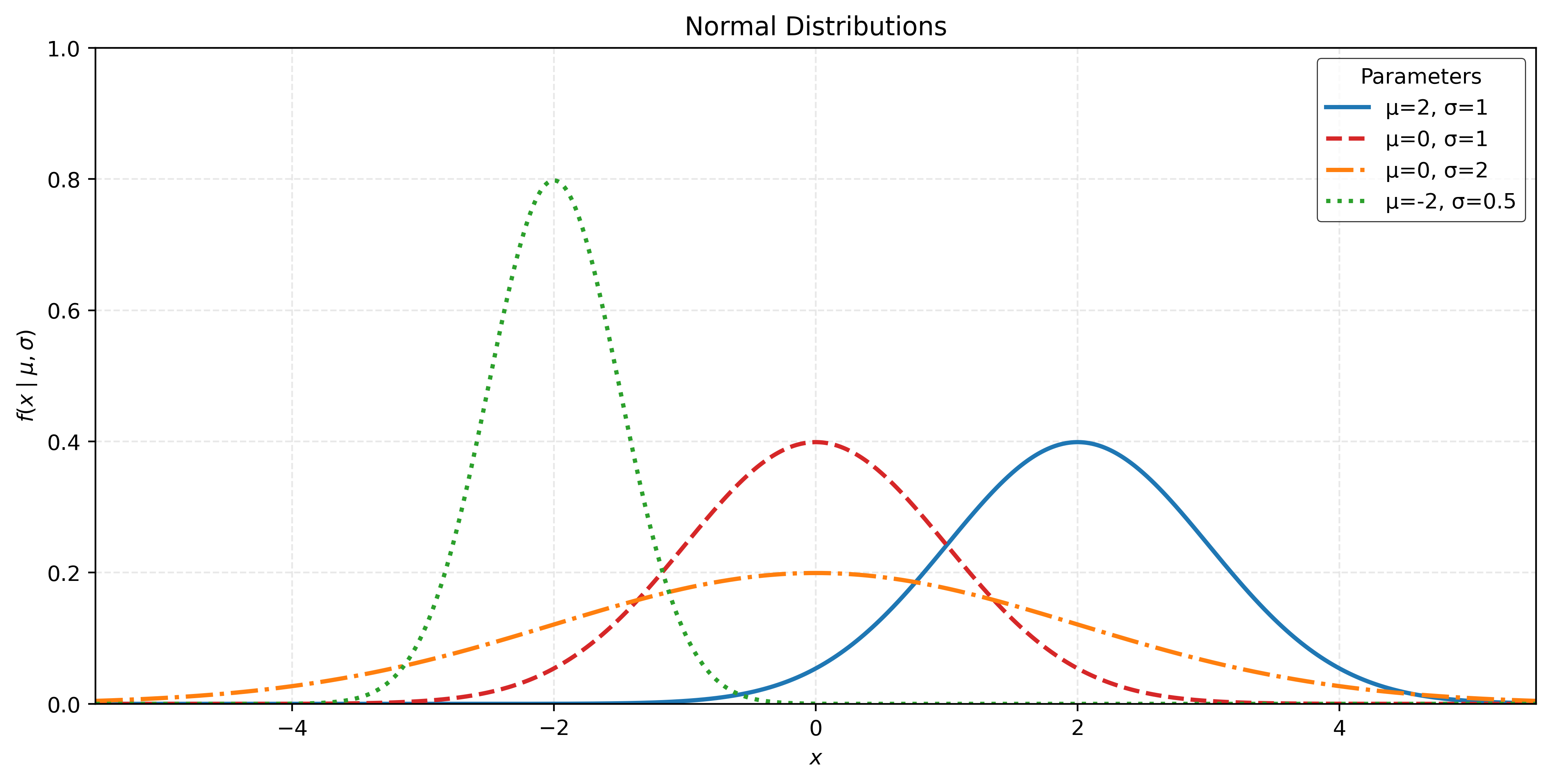
Estimation
Given data \(x_1, x_2, \ldots, x_n\) that is assumed to be an independent and identically distributed (i.i.d.) sample from a normal distribution with unknown mean \(\mu\) and unknown variance \(\sigma^2\) (thus standard deviation \(\sigma\)), how can we estimate \(\mu\) and \(\sigma^2\)? Said another way, how can we assume a normal probability model and fit that model to the data?
The maximum likelihood estimates (MLE) of \(\mu\) and \(\sigma^2\) are given by:
\[ \hat{\mu} = \frac{1}{n} \sum_{i=1}^{n} x_i \]
\[ \hat{\sigma}^2 = \frac{1}{n} \sum_{i=1}^{n} (x_i - \hat{\mu})^2 \]
Taking a square root gives the MLE of \(\sigma\):
\[ \hat{\sigma} = \sqrt{\frac{1}{n} \sum_{i=1}^{n} (x_i - \hat{\mu})^2} \]
The maximum likelihood estimates are found by maximizing the likelihood, which is the product of the PDF at each data point, however with unknown parameter values.
\[ \mathcal{L}(\theta \mid x_1, x_2, \ldots, x_n) = \prod_{i=1}^{n} f(x_i \mid \theta) \]
In the case of the normal distribution, the likelihood is:
\[ \mathcal{L}(\mu, \sigma^2 \mid x_1, x_2, \ldots, x_n) = \prod_{i=1}^{n} f(x_i \mid \mu, \sigma^2) = \prod_{i=1}^{n} \frac{1}{\sqrt{2\pi\sigma^2}} \exp\left(-\frac{(x_i - \mu)^2}{2\sigma^2}\right) \]
Maximizing the likelihood is equivalent to maximizing the log-likelihood, which is given by:
\[ \begin{align} \ell(\mu, \sigma^2 \mid x_1, x_2, \ldots, x_n) &= \log \left (\mathcal{L}(\mu, \sigma^2 \mid x_1, x_2, \ldots, x_n)\right) \\ &= \sum_{i=1}^{n} \log f(x_i \mid \mu, \sigma^2) \\ &= \sum_{i=1}^{n} \left[-\frac{1}{2}\log(2\pi) - \frac{1}{2}\log(\sigma^2) - \frac{(x_i - \mu)^2}{2\sigma^2}\right] \end{align} \]
Note that the log of the product is the sum of the logs. Maximizing the log-likelihood is preferred as it is often easier to work with for optimization.
Here we can simplify the log-likelihood further.
\[ \ell(\mu, \sigma^2 \mid x_1, x_2, \ldots, x_n) = -\frac{n}{2}\log(2\pi) - \frac{n}{2}\log(\sigma^2) - \frac{1}{2\sigma^2}\sum_{i=1}^{n} (x_i - \mu)^2 \]
From here, we want to find the values of \(\mu\) and \(\sigma^2\) that maximize this log-likelihood. Importantly, while likelihoods are based on density functions, likelihoods assume that the data is known and the parameters are unknown. This is the opposite of the density function, which assumes that the parameters are known and the data is unknown.
Completing the optimization, we would find the MLE stated above.
\[ \hat{\mu} = \frac{1}{n} \sum_{i=1}^{n} x_i \]
\[ \hat{\sigma}^2 = \frac{1}{n} \sum_{i=1}^{n} (x_i - \hat{\mu})^2 \]
Show Code for Plot
# generate some data from a single normal distribution
np.random.seed(42)
data = np.random.normal(loc=4, scale=1.5, size=200)

# "fit" three normals to the data with different parameters
mu_estimates = [3.5, 4.0, 4.5]
sigma_estimates = [1.0, 1.5, 2.0]

# calculate log-likelihoods for each fitted normal
log_likelihoods = []
for mu, sigma in zip(mu_estimates, sigma_estimates):
    log_likelihood = np.sum(norm.logpdf(data, loc=mu, scale=sigma))
    log_likelihoods.append(log_likelihood)

# plot the data and fitted normals
fig, ax = plt.subplots(figsize=(10, 6))
sns.rugplot(data, ax=ax, color="tab:red", alpha=0.5, expand_margins=False)

x = np.linspace(data.min() - 1, data.max() + 1, 1000)
colors = ["tab:blue", "tab:orange", "tab:green"]
lines = ["-", "--", "-.", ":"]

for mu, sigma, color, line, log_likelihood in zip(
    mu_estimates, sigma_estimates, colors, lines, log_likelihoods
):
    ax.plot(
        x,
        norm.pdf(x, loc=mu, scale=sigma),
        color=color,
        label=f"Log-Likelihood={log_likelihood:.2f}",
        linestyle=line,
    )

ax.set_title("Rug Plot with Fitted Normals")
ax.set_xlabel("Data")
ax.set_ylabel("Density")
ax.legend(title="Fitted Normals")
ax.grid(color="lightgrey", linestyle="--")
plt.show()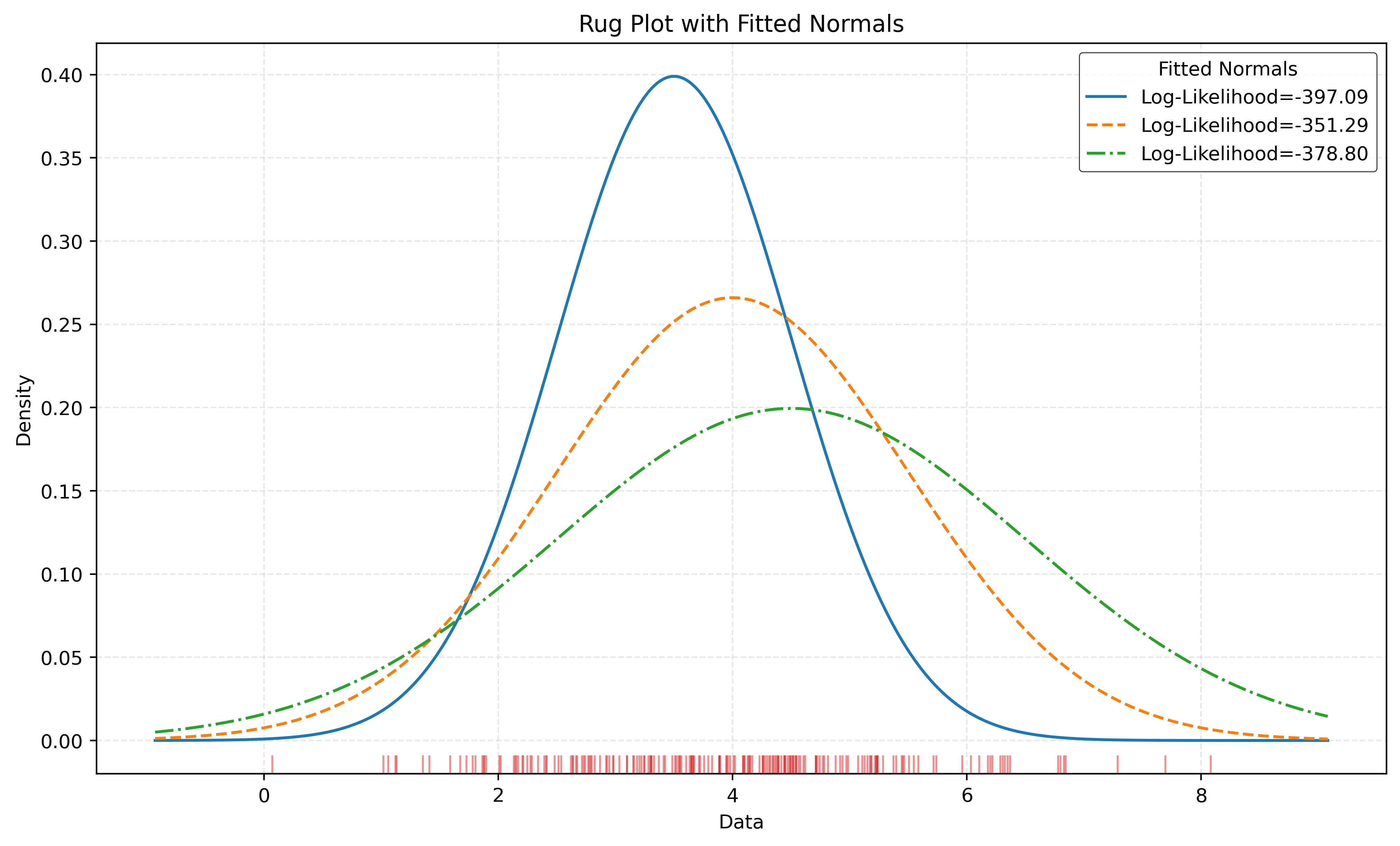
Some Bayes Theorem
Given priors:
- \(\pi_A = P(Y = A) = 0.20\)
- \(\pi_B = P(Y = B) = 0.50\)
- \(\pi_C = P(Y = C) = 0.30\)
And likelihoods:
- \(X \mid Y = A \sim N(\mu = 2, \sigma = 1)\)
- \(X \mid Y = B \sim N(\mu = 3, \sigma = 2)\)
- \(X \mid Y = C \sim N(\mu = 4, \sigma = 1)\)
Calculate posteriors:
- \(P(Y = A \mid X = 3.4)\)
- \(P(Y = B \mid X = 3.4)\)
- \(P(Y = C \mid X = 3.4)\)
Show Code for Plot
x = np.linspace(-2, 8, 1000)
classes = ["A", "B", "C"]
mu = [2, 3, 4]
sigma = [1, 2, 1]

fig, axs = plt.subplots(1, 2, figsize=(12, 5))

for i in range(3):
    y = norm.pdf(x, loc=mu[i], scale=sigma[i])
    axs[0].plot(x, y, label=f"Y={classes[i]}", linewidth=2)

axs[0].axvline(x=3.4, color="red", linestyle="--")
axs[0].set_xlabel("X")
axs[0].set_ylabel("Density")
axs[0].grid(color="lightgrey", linestyle="--")
axs[0].set_title("Likelihoods")
axs[0].legend()

priors = [0.20, 0.50, 0.30]

z = []
for i in range(len(x)):
    z.append(np.sum(priors * norm.pdf(x[i], loc=mu, scale=sigma)))

for i in range(3):
    y = priors[i] * norm.pdf(x, loc=mu[i], scale=sigma[i])
    axs[1].plot(x, y / z, label=f"Y={classes[i]}", linewidth=2)

axs[1].axvline(x=3.4, color="red", linestyle="--")
axs[1].set_xlabel("X")
axs[1].set_ylabel("Density")
axs[1].grid(color="lightgrey", linestyle="--")
axs[1].set_title("Posteriors")
axs[1].legend()

plt.show()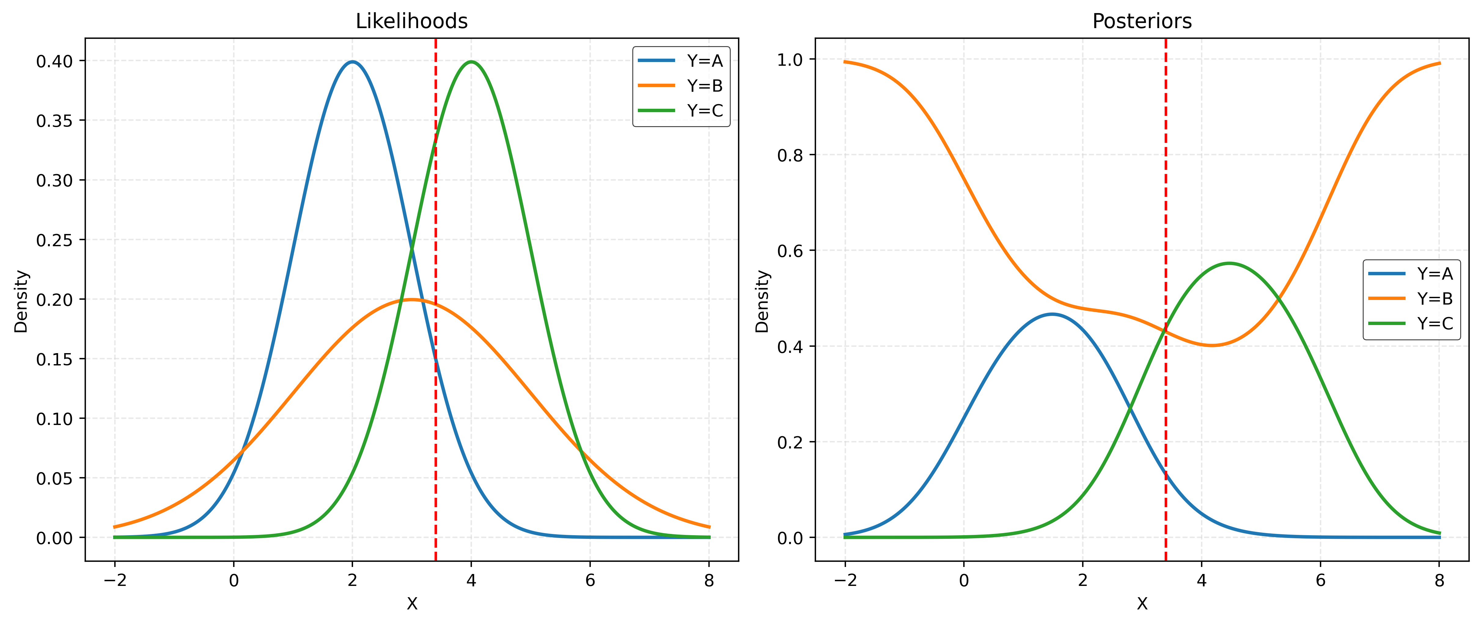
priors = [0.20, 0.50, 0.30]
likelihoods = norm.pdf(x=3.4, loc=[2, 3, 4], scale=[1, 2, 1])
priors * likelihoods / (np.sum(priors * likelihoods))
array([0.1315, 0.4294, 0.4391])- \(P(Y = A \mid X = 3.7) = 0.13152821\)
- \(P(Y = B \mid X = 3.7) = 0.42938969\)
- \(P(Y = C \mid X = 3.7) = 0.43908211\)
Generative Models
\[ p_k(\pmb{x}) = P(Y = k \mid \pmb{X} = \pmb{x}) = \frac{\pi_k \cdot f_k(\pmb{x})}{\sum_{g = 1}^{G} \pi_g \cdot f_g(\pmb{x})} \]
Helper Functions
def make_plot(mu1, cov1, mu2, cov2, seed=42):

    # control random sampling
    np.random.seed(seed)

    # create two multivariate normal distributions
    dist1 = multivariate_normal(mu1, cov1)
    dist2 = multivariate_normal(mu2, cov2)

    # generate random samples from each distribution
    samples1 = dist1.rvs(size=100)
    samples2 = dist2.rvs(size=100)

    # change color maps for scatter plot
    cmap1 = plt.get_cmap("Blues")
    cmap2 = plt.get_cmap("Oranges")

    # arrange plot grid points
    x_min = np.min([np.min(samples1[:, 0]), np.min(samples2[:, 0])]) - 1
    x_max = np.max([np.max(samples1[:, 0]), np.max(samples2[:, 0])]) + 1
    y_min = np.min([np.min(samples1[:, 1]), np.min(samples2[:, 1])]) - 1
    y_max = np.max([np.max(samples1[:, 1]), np.max(samples2[:, 1])]) + 1
    x, y = np.mgrid[x_min:x_max:0.01, y_min:y_max:0.01]
    pos = np.empty(x.shape + (2,))
    pos[:, :, 0] = x
    pos[:, :, 1] = y

    # setup plots
    fig, ax = plt.subplots(1, 2, figsize=(10, 5))

    # plot true distributions
    ax[0].contourf(x, y, dist1.pdf(pos), cmap="Blues")
    ax[0].contour(x, y, dist1.pdf(pos), colors="k")
    ax[0].contourf(x, y, dist2.pdf(pos), cmap="Oranges", alpha=0.5)
    ax[0].contour(x, y, dist2.pdf(pos), colors="k")
    ax[0].grid(color="lightgrey", linestyle="--")
    ax[0].set_title("True Distribution")
    ax[0].set_xlabel(r"$x_1$")
    ax[0].set_ylabel(r"$x_2$")

    # plot sampled data
    ax[1].scatter(samples1[:, 0], samples1[:, 1], color=cmap1(0.5))
    ax[1].scatter(samples2[:, 0], samples2[:, 1], color=cmap2(0.5))
    ax[1].set_title("Sampled Data")
    ax[1].grid(color="lightgrey", linestyle="--")
    ax[0].set_xlim(x_min, x_max)
    ax[0].set_ylim(y_min, y_max)
    ax[1].set_xlim(x_min, x_max)
    ax[1].set_ylim(y_min, y_max)
    ax[1].set_xlabel(r"$x_1$")
    ax[1].set_ylabel(r"$x_2$")

    # shot plot
    plt.show()
# create mean (mu) and covariance (cov) arrays
def create_params(mu_1, mu_2, sigma_1, sigma_2, corr):
# Create mean vector
mu = np.array([mu_1, mu_2])
# Calculate covariance matrix
cov = np.array(
[
[sigma_1**2, corr * sigma_1 * sigma_2],
[corr * sigma_1 * sigma_2, sigma_2**2],
]
)
# Return both
return mu, cov# print parameter information
def print_setup_parameter_info(mu1, cov1, mu2, cov2):
print("Mean X when Y = Blue:", mu1)
print("Covariance of X when Y = Blue:", "\n", cov1)
print("Mean X when Y = Orange:", mu2)
print("Covariance of X when Y = Orange:", "\n", cov2)Linear Discriminant Analysis (LDA)
Linear Discriminant Analysis, LDA, assumes that the features are multivariate normal conditioned on the target classes. Importantly, LDA assumes the same covariance (shape) within each class.
\[ \pmb{X} \mid Y = k \sim N(\pmb{\mu}_k, \Sigma) \]
\[ \Sigma = \Sigma_1 = \Sigma_2 = \cdots = \Sigma_G \]
# make a two-class LDA setup
mu1, cov1 = create_params(0, 0, 1, 1, 0.5)
mu2, cov2 = create_params(2, 2, 1, 1, 0.5)
print_setup_parameter_info(mu1, cov1, mu2, cov2)
Mean X when Y = Blue: [0 0]
Covariance of X when Y = Blue:
[[1. 0.5]
[0.5 1. ]]
Mean X when Y = Orange: [2 2]
Covariance of X when Y = Orange:
[[1. 0.5]
[0.5 1. ]]# plot (true) conditional distributions of X and sampled data
make_plot(mu1, cov1, mu2, cov2)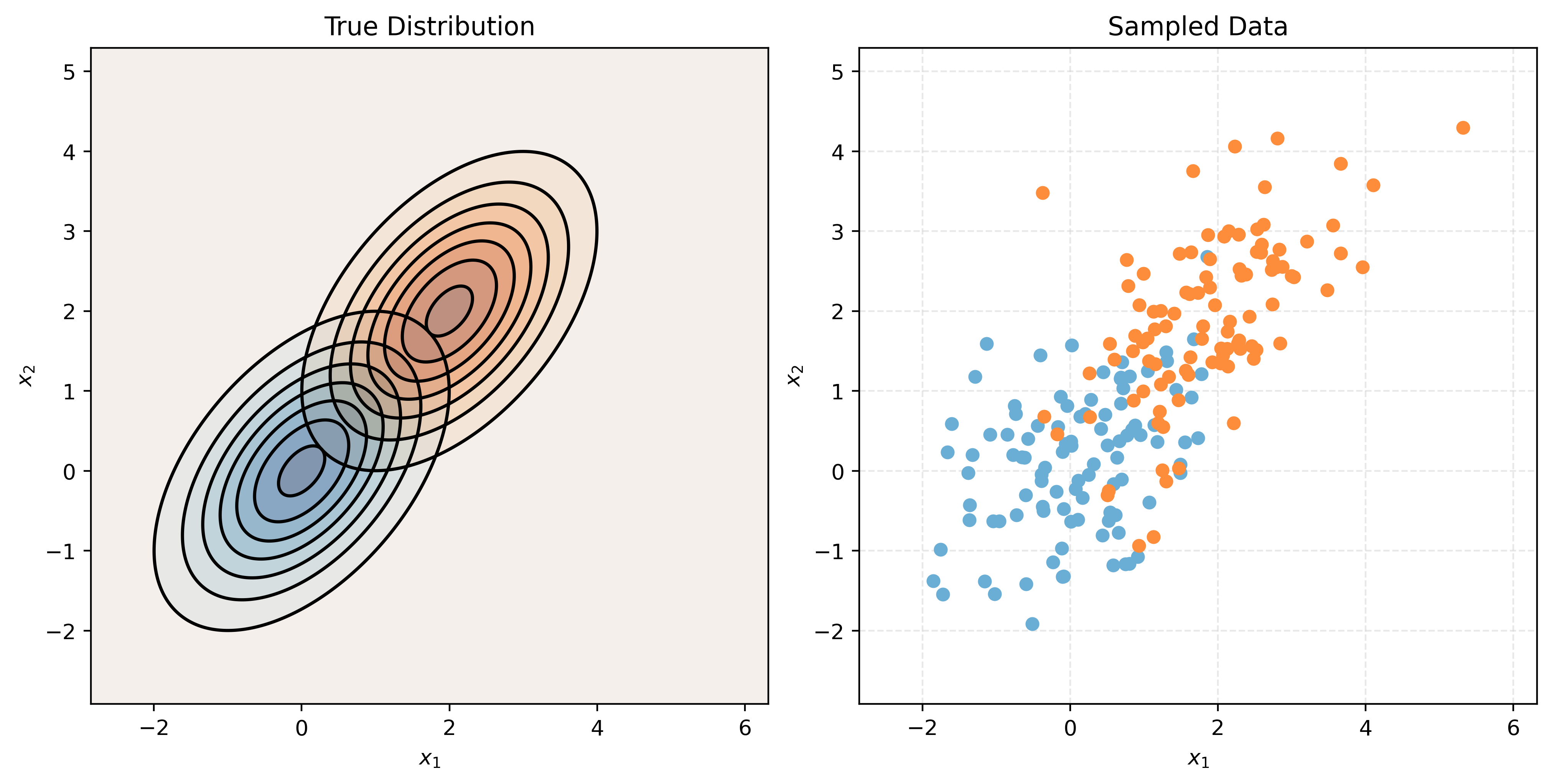
Quadratic Discriminant Analysis (QDA)
Quadratic Discriminant Analysis, QDA, also assumes that the features are multivariate normal conditioned on the target classes. However, unlike LDA, QDA makes fewer assumptions on the covariances (shapes). QDA allows the covariance to be completely different within each class.
\[ \pmb{X} \mid Y = k \sim N(\pmb{\mu}_k, \Sigma_k) \]
# make a two-class QDA setup
mu1, cov1 = create_params(0, 0, 2, 1, 0.5)
mu2, cov2 = create_params(2, 2, 1, 0.5, -0.5)
print_setup_parameter_info(mu1, cov1, mu2, cov2)
Mean X when Y = Blue: [0 0]
Covariance of X when Y = Blue:
[[4. 1.]
[1. 1.]]
Mean X when Y = Orange: [2 2]
Covariance of X when Y = Orange:
[[ 1. -0.25]
[-0.25 0.25]]# plot (true) conditional distributions of X and sampled data
make_plot(mu1, cov1, mu2, cov2)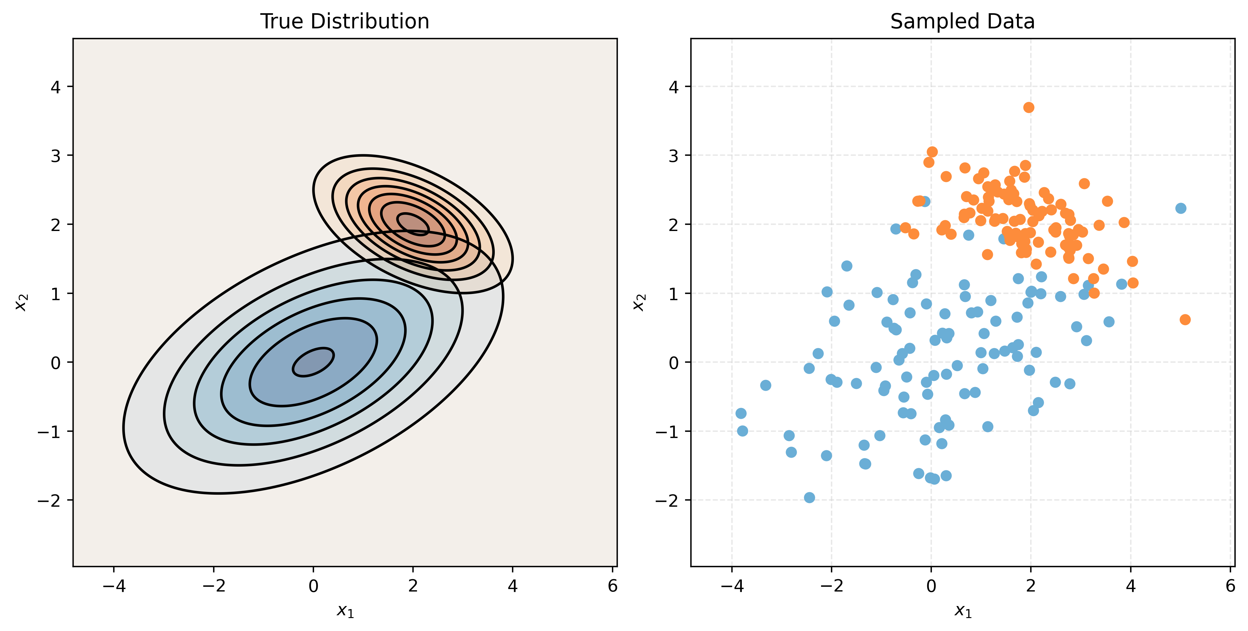
Naive Bayes (NB)
Naive Bayes comes in many forms. With only numeric features, it often assumes a multivariate normal conditioned on the target classes, but a very specific multivariate normal.
\[ {\pmb{X}} \mid Y = k \sim N(\pmb{\mu}_k, \Sigma_k) \]
Naive Bayes assumes that the features \(X_1, X_2, \ldots, X_p\) are independent given \(Y = k\). This is the “naive” part of naive Bayes. The Bayes part is nothing new. Since \(X_1, X_2, \ldots, X_p\) are assumed independent, each \(\Sigma_k\) is diagonal, that is, we assume no correlation between features. Independence implies zero correlation.
\[ \Sigma_k = \begin{bmatrix} \sigma_{1}^2 & 0 & \cdots & 0 \\ 0 & \ddots & \ddots & \vdots \\ \vdots & \ddots & \ddots & 0 \\ 0 & \cdots & 0 & \sigma_{p}^2 \\ \end{bmatrix} \]
This will allow us to write the (joint) likelihood as a product of univariate distributions. In this case, the product of univariate normal distributions instead of a (joint) multivariate distribution.
\[ f_k(\pmb{x}) = \prod_{j = 1}^{p} f_{kj}(x_j) \]
Here, \(f_{kj}(x_j)\) is the density for the \(j\)-th feature conditioned on the \(k\)-th class. Notice that there is a \(\sigma_{kj}\) for each feature for each class.
\[ f_{kj}(x_j) = \frac{1}{\sigma_{kj}\sqrt{2\pi}}\exp\left[-\frac{1}{2}\left(\frac{x_j - \mu_{kj}}{\sigma_{kj}}\right)^2\right] \]
When \(p = 1\), this version of naive Bayes is equivalent to QDA.
# make a two-class NB setup
mu1, cov1 = create_params(0, 0, 2, 1, 0)
mu2, cov2 = create_params(2, 2, 1, 0.5, 0)
print_setup_parameter_info(mu1, cov1, mu2, cov2)
Mean X when Y = Blue: [0 0]
Covariance of X when Y = Blue:
[[4 0]
[0 1]]
Mean X when Y = Orange: [2 2]
Covariance of X when Y = Orange:
[[1. 0. ]
[0. 0.25]]# plot (true) conditional distributions of X and sampled data
make_plot(mu1, cov1, mu2, cov2)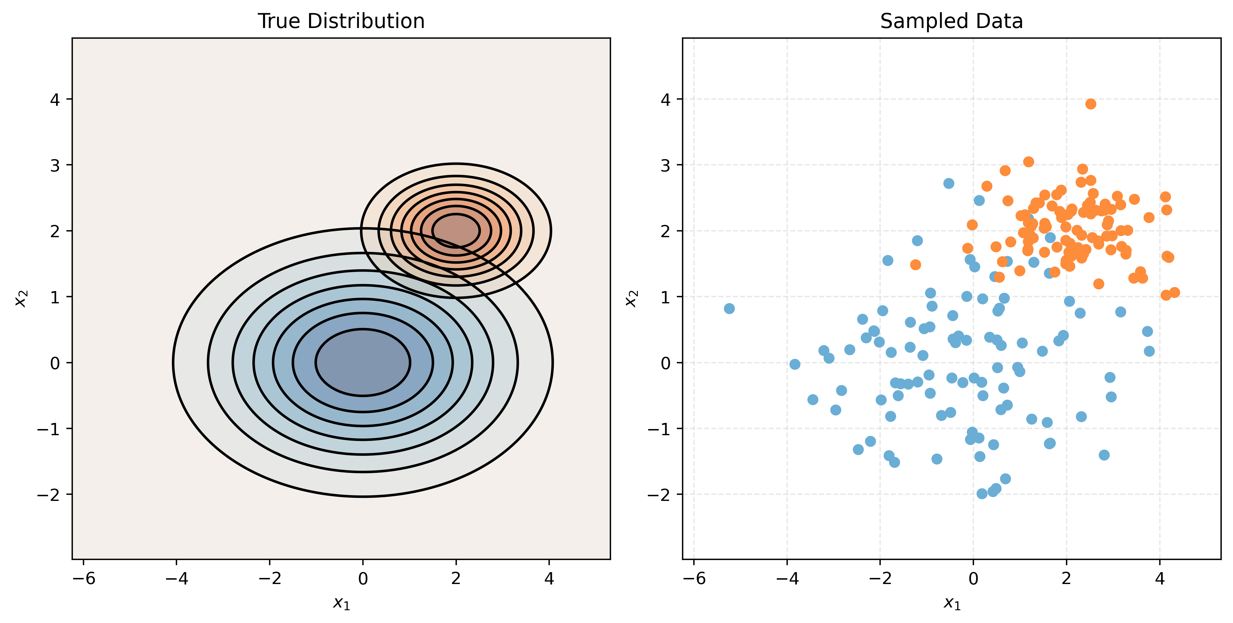
Generative Models with sklearn
# function to generate data according to LDA, QDA, or NB
def generate_data(n1, n2, n3, mu1, mu2, mu3, cov1, cov2, cov3, seed=307):

    # control random sampling
    np.random.seed(seed)

    # generate data for class A
    data1 = np.random.multivariate_normal(mu1, cov1, n1)
    labels1 = np.repeat("A", n1)

    # generate data for class B
    data2 = np.random.multivariate_normal(mu2, cov2, n2)
    labels2 = np.repeat("B", n2)

    # generate data for class C
    data3 = np.random.multivariate_normal(mu3, cov3, n3)
    labels3 = np.repeat("C", n3)

    # combine data and labels
    data = np.concatenate((data1, data2, data3))
    labels = np.concatenate((labels1, labels2, labels3))

    # make X and y
    X = pd.DataFrame(data, columns=["x1", "x2"])
    y = pd.Series(labels)

    return X, y
# setup sample sizes
n1 = 500
n2 = 500
n3 = 500
# setup parameters
mu1, cov1 = create_params(0, 0, 2, 1, 0.5)
mu2, cov2 = create_params(2, 2, 1, 2, -0.5)
mu3, cov3 = create_params(0, 2, 1, 1, 0.5)# generate train and test data
X_train, y_train = generate_data(n1, n2, n3, mu1, mu2, mu3, cov1, cov2, cov3)
X_test, y_test = generate_data(n1, n2, n3, mu1, mu2, mu3, cov1, cov2, cov3)# plot the train data
p = sns.jointplot(x="x1", y="x2", data=X_train, hue=y_train, space=0)
p.figure.suptitle("Simulated Train Data", y=1.01)
p.figure.set_size_inches(8, 8)
plt.show()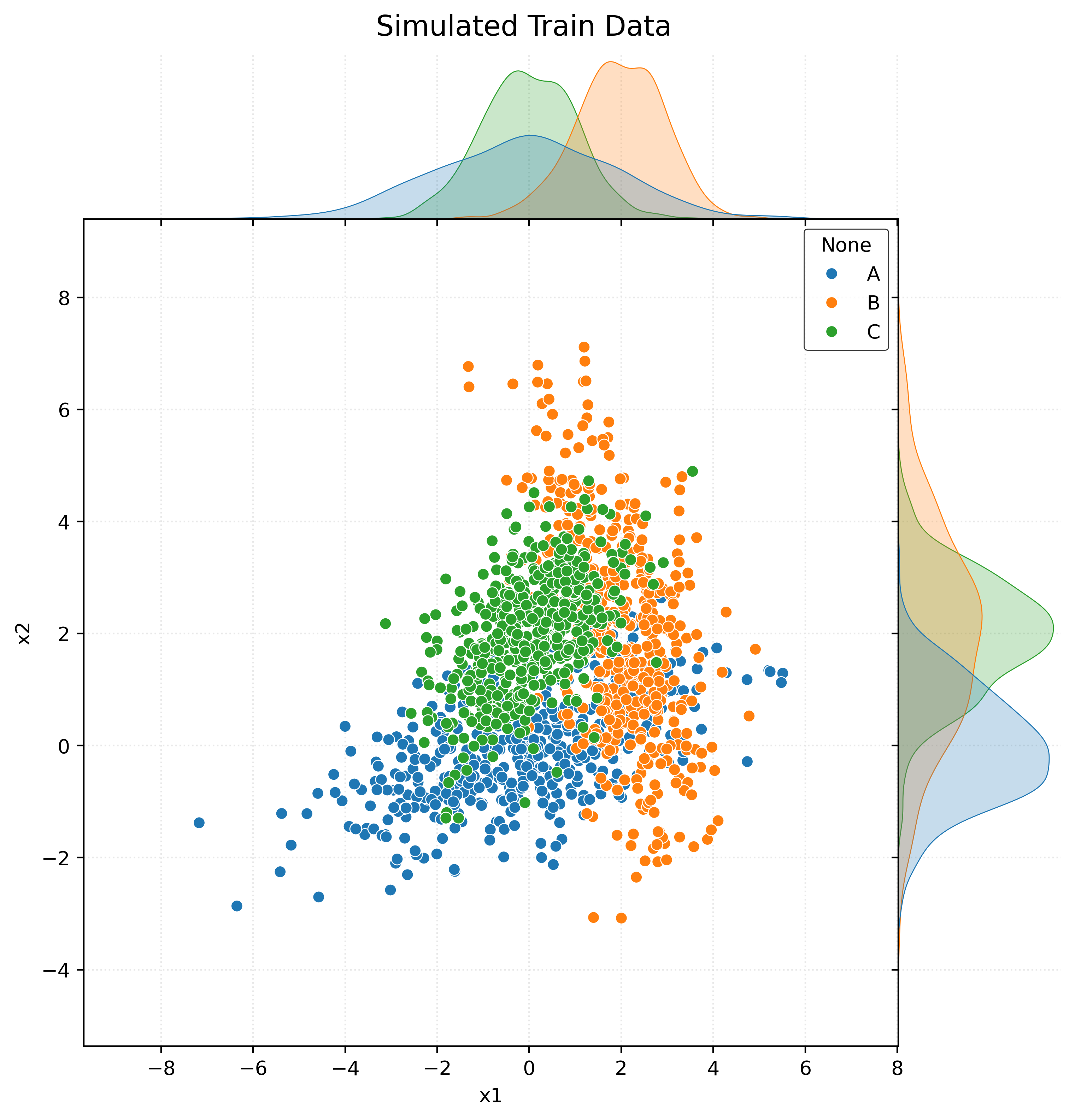
# (gaussian) naive bayes
gnb = GaussianNB()
gnb.fit(X_train, y_train)
y_pred = gnb.predict(X_test)
accuracy = accuracy_score(y_test, y_pred)
print("Gaussian NB, Test Accuracy:", accuracy)

# linear discriminant analysis
lda = LinearDiscriminantAnalysis(store_covariance=True)
lda.fit(X_train, y_train)
y_pred = lda.predict(X_test)
accuracy = accuracy_score(y_test, y_pred)
print("LDA, Test Accuracy:", accuracy)

# quadratic discriminant analysis
qda = QuadraticDiscriminantAnalysis(store_covariance=True)
qda.fit(X_train, y_train)
y_pred = qda.predict(X_test)
accuracy = accuracy_score(y_test, y_pred)
print("QDA, Test Accuracy:", accuracy)
Gaussian NB, Test Accuracy: 0.7573333333333333
LDA, Test Accuracy: 0.7166666666666667
QDA, Test Accuracy: 0.778print("Classes:", gnb.classes_)
print("Feature names:", gnb.feature_names_in_)
print("NB, Estimated Class Priors:", gnb.class_prior_)
print("NB, Estimated Mean of each feature per class:", "\n", gnb.theta_)
print("NB, Estimated Variance of each feature per class:", "\n", gnb.var_)Classes: ['A' 'B' 'C']
Feature names: ['x1' 'x2']
NB, Estimated Class Priors: [0.3333 0.3333 0.3333]
NB, Estimated Mean of each feature per class:
[[-0.1078 -0.0255]
[ 1.9638 2.022 ]
[-0.0045 1.9877]]
NB, Estimated Variance of each feature per class:
[[3.8624 0.9592]
[0.9138 3.4717]
[1.0168 1.0249]]print("Classes:", lda.classes_)
print("Feature names:", lda.feature_names_in_)
print("LDA, Estimated Class Priors:", lda.priors_)
print("LDA, Estimated Mean of each feature per class:", "\n", lda.means_)
print("LDA, Estimated Covariance Matrix:")
lda.covariance_Classes: ['A' 'B' 'C']
Feature names: ['x1' 'x2']
LDA, Estimated Class Priors: [0.3333 0.3333 0.3333]
LDA, Estimated Mean of each feature per class:
[[-0.1078 -0.0255]
[ 1.9638 2.022 ]
[-0.0045 1.9877]]
LDA, Estimated Covariance Matrix:array([[1.931 , 0.2267],
[0.2267, 1.8186]])print("Classes:", qda.classes_)
print("Feature names:", qda.feature_names_in_)
print("QDA, Estimated Class Priors:", qda.priors_)
print("QDA, Estimated Mean of each feature per class:", "\n", qda.means_)
print("QDA, Estimated Covariance Matrix of each feature per class:")
qda.covariance_Classes: ['A' 'B' 'C']
Feature names: ['x1' 'x2']
QDA, Estimated Class Priors: [0.3333 0.3333 0.3333]
QDA, Estimated Mean of each feature per class:
[[-0.1078 -0.0255]
[ 1.9638 2.022 ]
[-0.0045 1.9877]]
QDA, Estimated Covariance Matrix of each feature per class:[array([[3.8701, 1.0502],
[1.0502, 0.9612]]),
array([[ 0.9157, -0.872 ],
[-0.872 , 3.4786]]),
array([[1.0188, 0.5032],
[0.5032, 1.027 ]])]Priors
# setup sample sizes
n1_train = 500
n2_train = 300
n3_train = 700
n1_test = 500
n2_test = 500
n3_test = 500

# setup parameters
mu1, cov1 = create_params(0, 0, 2, 1, 0.5)
mu2, cov2 = create_params(2, 2, 1, 2, -0.5)
mu3, cov3 = create_params(0, 2, 1, 1, 0.5)

# generate train and test data
X_train, y_train = generate_data(n1_train, n2_train, n3_train, mu1, mu2, mu3, cov1, cov2, cov3)
X_test, y_test = generate_data(n1_test, n2_test, n3_test, mu1, mu2, mu3, cov1, cov2, cov3)
# quadratic discriminant analysis, estimated prior
qda = QuadraticDiscriminantAnalysis(
store_covariance=True,
)
qda.fit(X_train, y_train)
y_pred = qda.predict(X_test)
accuracy = accuracy_score(y_test, y_pred)
print("QDA, Test Accuracy:", accuracy)
print(qda.priors_)QDA, Test Accuracy: 0.7626666666666667
[0.3333 0.2 0.4667]# quadratic discriminant analysis, specified prior
qda = QuadraticDiscriminantAnalysis(
priors=[0.33, 0.33, 0.33],
store_covariance=True,
)
qda.fit(X_train, y_train)
y_pred = qda.predict(X_test)
accuracy = accuracy_score(y_test, y_pred)
print("QDA, Test Accuracy:", accuracy)
print(qda.priors_)QDA, Test Accuracy: 0.7773333333333333
[0.33 0.33 0.33]Footnotes
The use of \(n-1\) instead of \(n\) is known as Bessel’s correction.↩︎
However, they are both biased due to Jensen’s inequality.↩︎