Classification Introduction

In these notes, we will discuss:

the supervised learning classification task,
the Bayes classifier,
\(k\)-nearest neighbors,
classification metrics,
and estimating conditional probabilities with a learned model.

Along the way, you should notice that except for the conditional probabilities, the process followed mirrors that of regression.

# basic imports
import numpy as np
import pandas as pd
import seaborn as sns
import matplotlib.pyplot as plt

# machine learning imports
from sklearn.model_selection import train_test_split
from sklearn.datasets import make_blobs
from sklearn.neighbors import KNeighborsClassifier
from sklearn.metrics import accuracy_score

The Goal of Classification

Like, regression, classification is a supervised learning task. However, while regression is concerned with predicting a numeric target variable, classification seeks to predicts a categorical target variable.

X, y = make_blobs(
    n_samples=800,
    n_features=2,
    centers=3,
    cluster_std=4.2,
    random_state=42,
)

X_train, X_test, y_train, y_test = train_test_split(
    X,
    y,
    test_size=0.20,
    random_state=42,
)

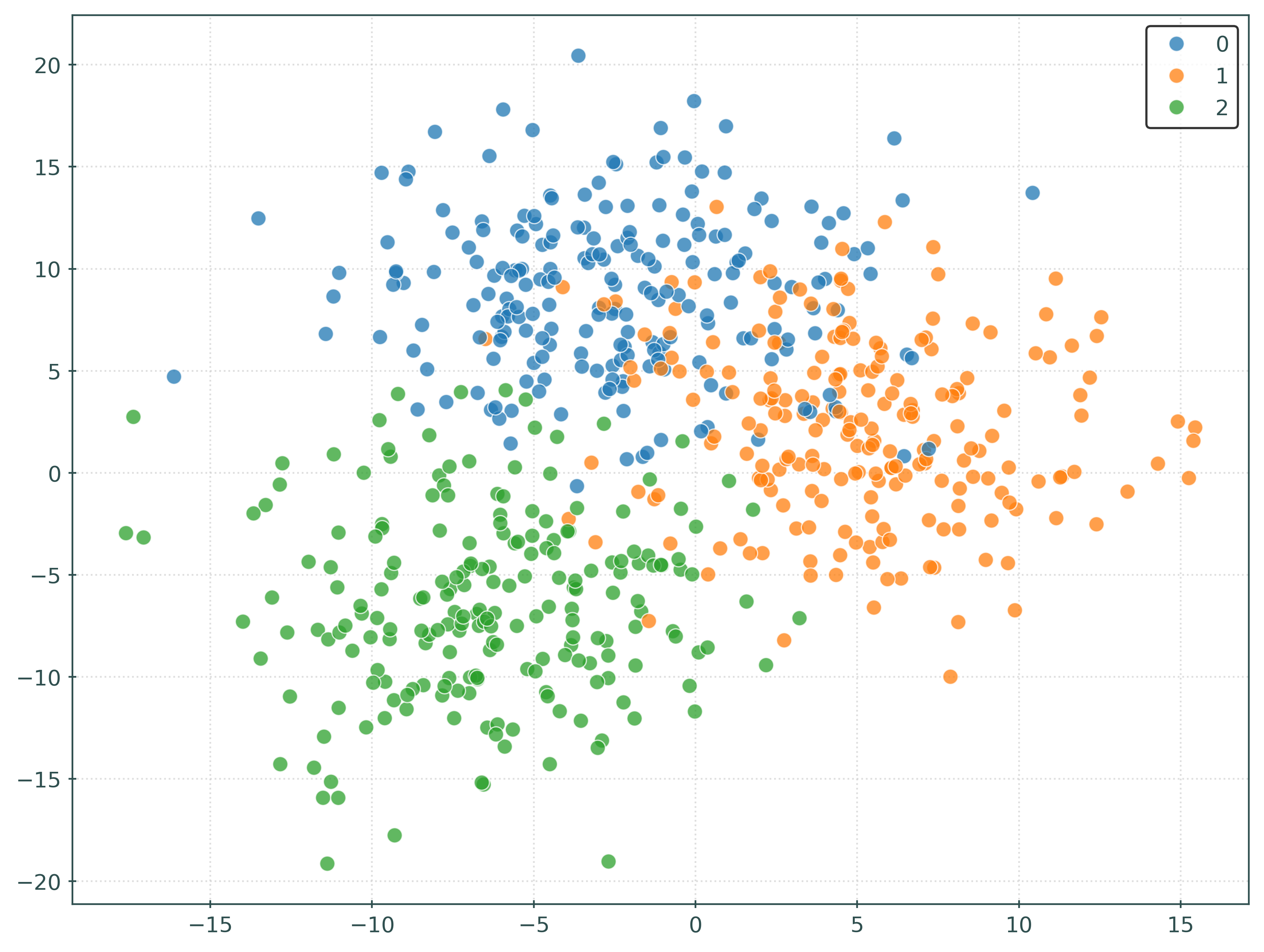
Show Code for Plot

fig, ax = plt.subplots()
fig.set_size_inches(8, 6)
scatter = sns.scatterplot(
    x=X_train[:, 0],
    y=X_train[:, 1],
    hue=y_train,
    palette="tab10",
    ax=ax,
    s=50,
    edgecolor="k",
    alpha=0.75,
)
ax.set_xlabel("$x_1$")
ax.set_ylabel("$x_2$")
ax.set_title("Simulated Training Data for Classification")
plt.show()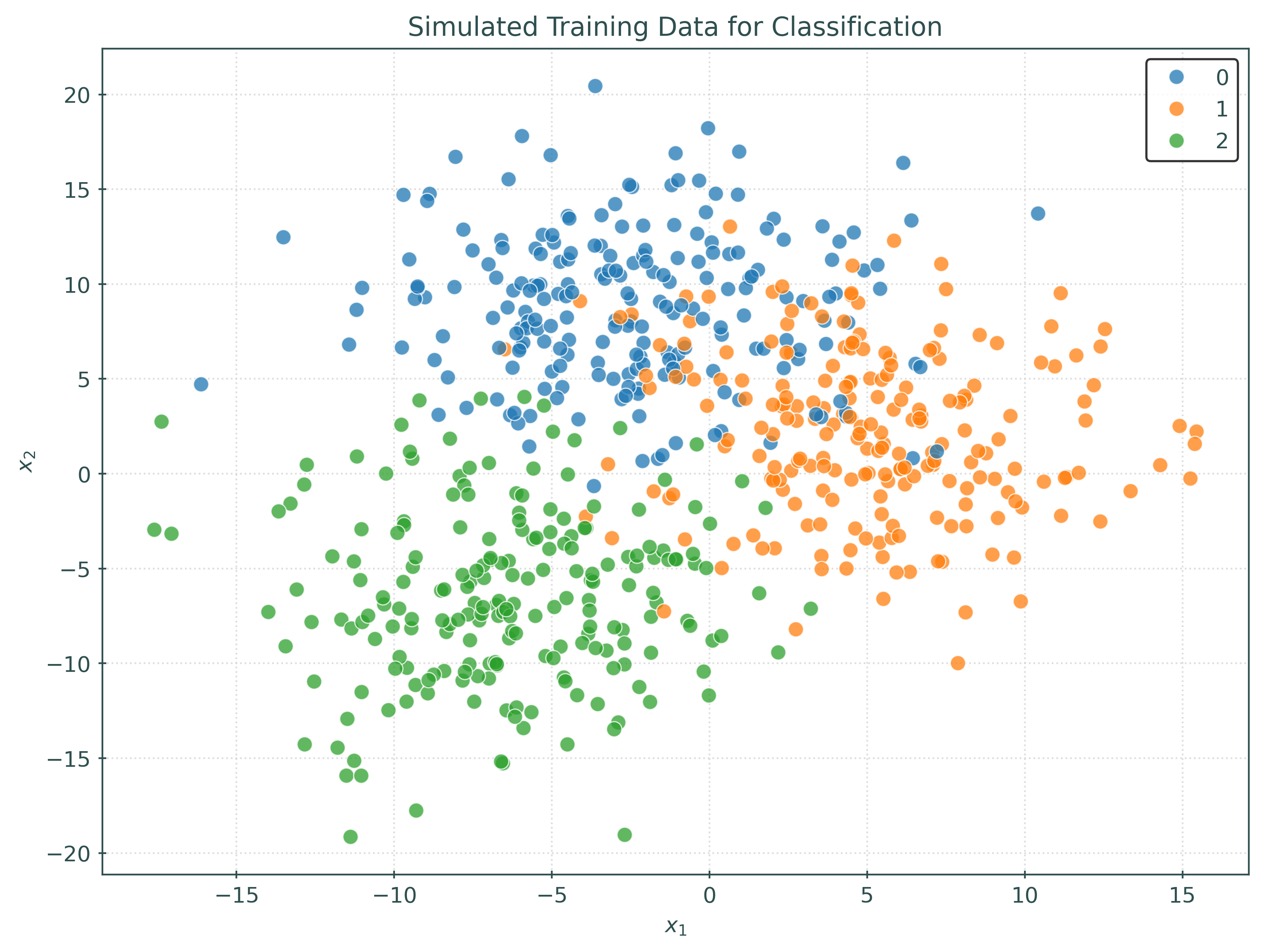

Consider new data at \(x = (x_1, x_2)\). The goal of classification is to predict the class label \(y\) for this new data point. Consider the following example when \(x = (-5, 5)\).

Show Code for Plot

fig, ax = plt.subplots()
fig.set_size_inches(8, 6)
scatter = sns.scatterplot(
    x=X_train[:, 0],
    y=X_train[:, 1],
    hue=y_train,
    palette="tab10",
    ax=ax,
    s=50,
    edgecolor="k",
    alpha=0.75,
)
ax.set_xlabel("$x_1$")
ax.set_ylabel("$x_2$")
ax.set_title("Simulated Training Data for Classification")
ax.plot(
    -5,
    5,
    marker="o",
    markersize=10,
    color="red",
)
plt.show()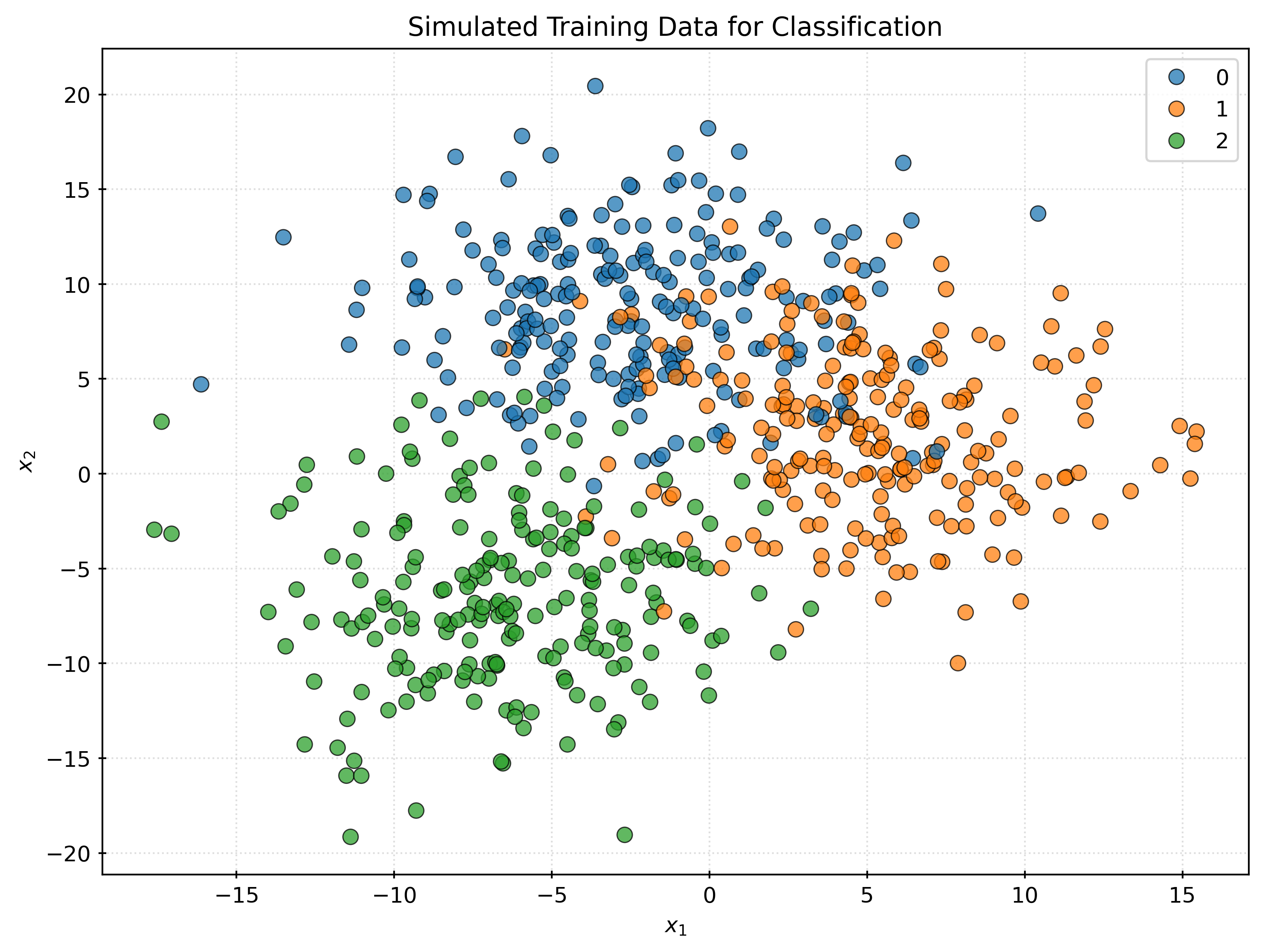

The fundamental question that classification seeks to answer is: what is the probability that \(Y = g\) given \(X = x\)?

So, in this case, what is the probability that:

\(Y = 0\) (blue) when \(x = (-5, 5)\)?
\(Y = 1\) (orange) when \(x = (-5, 5)\)?
\(Y = 2\) (green) when \(x = (-5, 5)\)?

With these questions answered, we can then make a prediction for the class label of \(x = (-5, 5)\). Simply predict the class label with the highest probability!

Unfortunately, we do not know the true conditional probabilities. So instead, we will fit a model that can be used to estimate these probabilities.

Bayes Classifier

The Bayes Classifier, \(C^B(x)\), is the classifier that minimizes the probability of misclassification, and thus is considered the optimal classifier. However, the Bayes Classifier cannot be used in practice as it requires knowledge of the true conditional probabilities. It is simply a useful concept for theoretical understanding of classification.

\[ p_g(x) = P\left[ Y = g \mid X = x \right] \]

\[ C^B(x) = \underset{g \in \{1, 2, \ldots G\}}{\text{argmax}} P\left[ Y = k \mid X = x \right] \]

The Bayes Classifier simply says “predict the class label with the highest conditional probability”.

Be aware that the Bayes Classifier is unrelated to the Naive Bayes Classifier that we will explore later.

Building a Classifier

Given that we cannot use the Bayes Classifier in practice, we will build a model that can be used to estimate the relevant conditional probabilities. With those estimate probabilities, we would then make predictions using the same rule as the Bayes Classifier, but with the estimated probabilities rather than known conditional probabilities.

\[ \hat{p}_g(x) = \hat{P}\left[ Y = k \mid X = x \right] \]

\[ \hat{C}(x) = \underset{g \in \{1, 2, \ldots G\}}{\text{argmax}} \hat{p}_g(x) \]

\(k\)-Nearest Neighbors

Our first model for classification will be the \(k\)-nearest neighbors classifier. Using \(k\)-nearest neighbors for classification is quite similar to \(k\)-nearest neighbors for regression.

After finding the \(k\)-nearest neighbors of \(x\), we will predict the class label of \(x\) as the class label that is most common among the \(k\)-nearest neighbors. More specifically, we can utilize the \(k\)-nearest neighbors to estimate the conditional probabilities. We will simply count the number of neighbors of each class label and divide by \(k\) to get the estimated probabilities!

\[ \hat{p}_g(x) = \hat{P}\left[ Y = k \mid X = x \right] = \frac{1}{k} \sum_{i \in \mathcal{N}_k(x)} I(y_i = g) \]

After estimating the conditional probabilities, we can then make a prediction for the class label of \(x\) that has the highest estimated conditional probability.

\[ \hat{C}(x) = \underset{g \in \{1, 2, \ldots G\}}{\text{argmax}} \hat{p}_g(x) \]

Like \(k\)-nearest neighbors regression, \(k\)-nearest neighbors for classification requires selecting a value for \(k\).

Metrics

There are many metrics to evaluate the performance of a classifier. We will detail a long list of them in the future. For introductory purposes, we will focus on two metrics: accuracy and misclassification.

\[ \text{Accuracy}(y, \hat{y}) = \frac{1}{n} \sum_{i=1}^{n} I(y_i = \hat{y}_i) \]

The accuracy is simply the proportion of correct predictions made by the classifier. We will see that accuracy is in many ways the default metric for classification, especially within sklearn.

Note that until RMSE for regression, which we want to minimize, accuracy is metric that we want to maximize. The classification error, or misclassification rate, is simply the proportion of incorrect predictions made by the classifier. So while these two metrics are related, and essentially measure the same thing, it can sometimes be useful to considered errors instead of correct predictions.

\[ \text{Misclassification}(y, \hat{y}) = \frac{1}{n} \sum_{i=1}^{n} I(y_i \neq \hat{y}_i) \]

\[ I(y_i = \hat{y}_i) = \begin{cases} 1 & \text{if } y_i = \hat{y}_i \\ 0 & \text{otherwise} \end{cases} \]

Example: Tuning a \(k\)-Nearest Neighbors Classifier

X_vtrain, X_validation, y_vtrain, y_validation = train_test_split(
    X_train,
    y_train,
    test_size=0.20,
    random_state=42,
)

k_values = range(1, 501, 10)
train_accuracies = []
validation_accuracies = []

for k in k_values:
    knn = KNeighborsClassifier(n_neighbors=k)
    knn.fit(X_vtrain, y_vtrain)
    y_pred_train = knn.predict(X_vtrain)
    y_pred_validation = knn.predict(X_validation)
    train_accuracy = accuracy_score(y_vtrain, y_pred_train)
    validation_accuracy = accuracy_score(y_validation, y_pred_validation)
    train_accuracies.append(train_accuracy)
    validation_accuracies.append(validation_accuracy)

best_k = k_values[np.argmax(validation_accuracies)]
print(f"Best k: {best_k}")
print(f"Validation Accuracy: {max(validation_accuracies):.2f}")

Best k: 201
Validation Accuracy: 0.87

validation_error = 1 - np.array(validation_accuracies)
train_error = 1 - np.array(train_accuracies)

fig, ax = plt.subplots()
fig.set_size_inches(8, 6)
ax.plot(
    k_values,
    train_error,
    label="Train Error",
    color="black",
    marker="o",
    markeredgecolor="black",
    markerfacecolor="tab:blue",
)
ax.plot(
    k_values,
    validation_error,
    label="Validation Error",
    color="black",
    marker="o",
    markeredgecolor="black",
    markerfacecolor="tab:orange",
)
ax.set_xlabel("k (Number of Neighbors)")
ax.set_ylabel("Error")
ax.set_title("Train and Validation Error versus k")
ax.invert_xaxis()
ax.legend()
plt.show()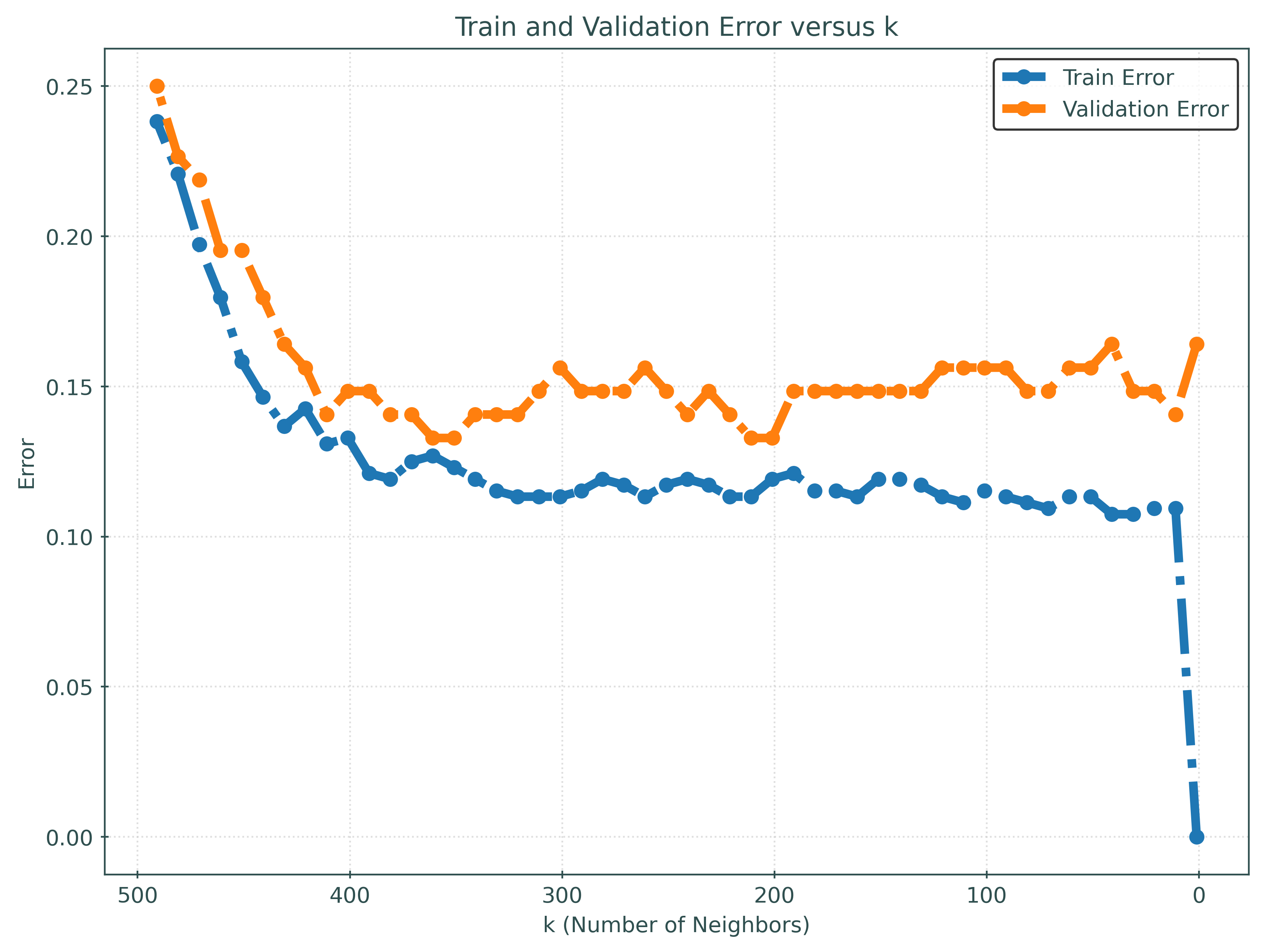

proportions = pd.Series(y_validation).value_counts(normalize=True)
print(proportions)

1   0.37
0   0.32
2   0.31
Name: proportion, dtype: float64

knn = KNeighborsClassifier(n_neighbors=best_k)
knn.fit(X_train, y_train)
y_pred_test = knn.predict(X_test)
test_accuracy = accuracy_score(y_test, y_pred_test)
print(f"Test Accuracy: {test_accuracy:.2f}")

Test Accuracy: 0.90

print(knn.predict_proba(X_test)[:10])

[[0.6119403  0.37313433 0.01492537]
 [0.10945274 0.80099502 0.08955224]
 [0.09950249 0.8358209  0.06467662]
 [0.0199005  0.04975124 0.93034826]
 [0.74626866 0.21890547 0.03482587]
 [0.72636816 0.27363184 0.        ]
 [0.74626866 0.08955224 0.1641791 ]
 [0.06467662 0.03482587 0.90049751]
 [0.06467662 0.53233831 0.40298507]
 [0.85074627 0.13930348 0.00995025]]

print(y_test[:10])

[1 1 1 2 0 0 0 2 1 0]

print(y_pred_test[:10])

[0 1 1 2 0 0 0 2 1 0]

results_df = pd.DataFrame(
    {
        "Actual": y_test[:10],
        "Predicted": y_pred_test[:10],
        
    }
)
prob_df = pd.DataFrame(knn.predict_proba(X_test)[:10])
prob_df.columns = [f"prob_{i}" for i in knn.classes_]
results_df = pd.concat([results_df, prob_df], axis=1)
print(results_df)

   Actual  Predicted  prob_0  prob_1  prob_2
0       1          0    0.61    0.37    0.01
1       1          1    0.11    0.80    0.09
2       1          1    0.10    0.84    0.06
3       2          2    0.02    0.05    0.93
4       0          0    0.75    0.22    0.03
5       0          0    0.73    0.27    0.00
6       0          0    0.75    0.09    0.16
7       2          2    0.06    0.03    0.90
8       1          1    0.06    0.53    0.40
9       0          0    0.85    0.14    0.01

The Goal of Classification

Bayes Classifier

Building a Classifier

\(k\)-Nearest Neighbors

Metrics

Example: Tuning a \(k\)-Nearest Neighbors Classifier

TODO