Neural Networks

This note is under active development. Some additional information can be found in the following scribbles.

• Neural Networks

Additionally, information specific to Convolutional Neural Networks (CNNs) can be found in the CNN Notebook at the end of this note.

# standard imports
import matplotlib.pyplot as plt
import numpy as np
import random

# sklearn data
from sklearn.datasets import make_blobs
from sklearn.datasets import make_circles
from sklearn.datasets import make_classification
from sklearn.datasets import load_digits
from sklearn.model_selection import train_test_split

# sklearn models
from sklearn.linear_model import LogisticRegression
from sklearn.ensemble import RandomForestClassifier

# sklearn metrics
from sklearn.metrics import accuracy_score
from sklearn.metrics import ConfusionMatrixDisplay

# pytorch imports
import torch
from torch import nn
from torch.utils.data import DataLoader
from torchvision import datasets
from torchvision.transforms import ToTensor

Torch Setup

# get cpu, gpu, or mps device for training
if torch.cuda.is_available():
    device = "cuda"
elif torch.backends.mps.is_available():
    device = "mps"
else:
    device = "cpu"

print(f"Using {device} device!")

Using cpu device!

If your machine does not allow for mps or cuda consider using:

• Google Colaboratory
  • Be sure to change the runtime type to a GPU.
• Illinois Computes Research Notebooks
  • Be sure to select the PyTorch option to utilize a GPU.

Logistic Regression as a Neural Network: Linear Data

# generate "linear" data
X, y = make_classification(
    n_samples=100,
    n_features=2,
    n_informative=2,
    n_redundant=0,
    n_clusters_per_class=1,
    random_state=2,
    n_classes=2,
)

# create a new figure and an axes
fig, ax = plt.subplots(figsize=(10, 6))

# plot the generated data
scatter = ax.scatter(
    X[:, 0],
    X[:, 1],
    c=y,
    cmap=plt.cm.Set1,
)

# set labels and title
ax.set_xlabel("Feature 1")
ax.set_ylabel("Feature 2")
ax.set_title("Linear Data")

# add a grid
ax.grid(
    color="lightgrey",
    linestyle="--",
)

# display the plot
plt.show()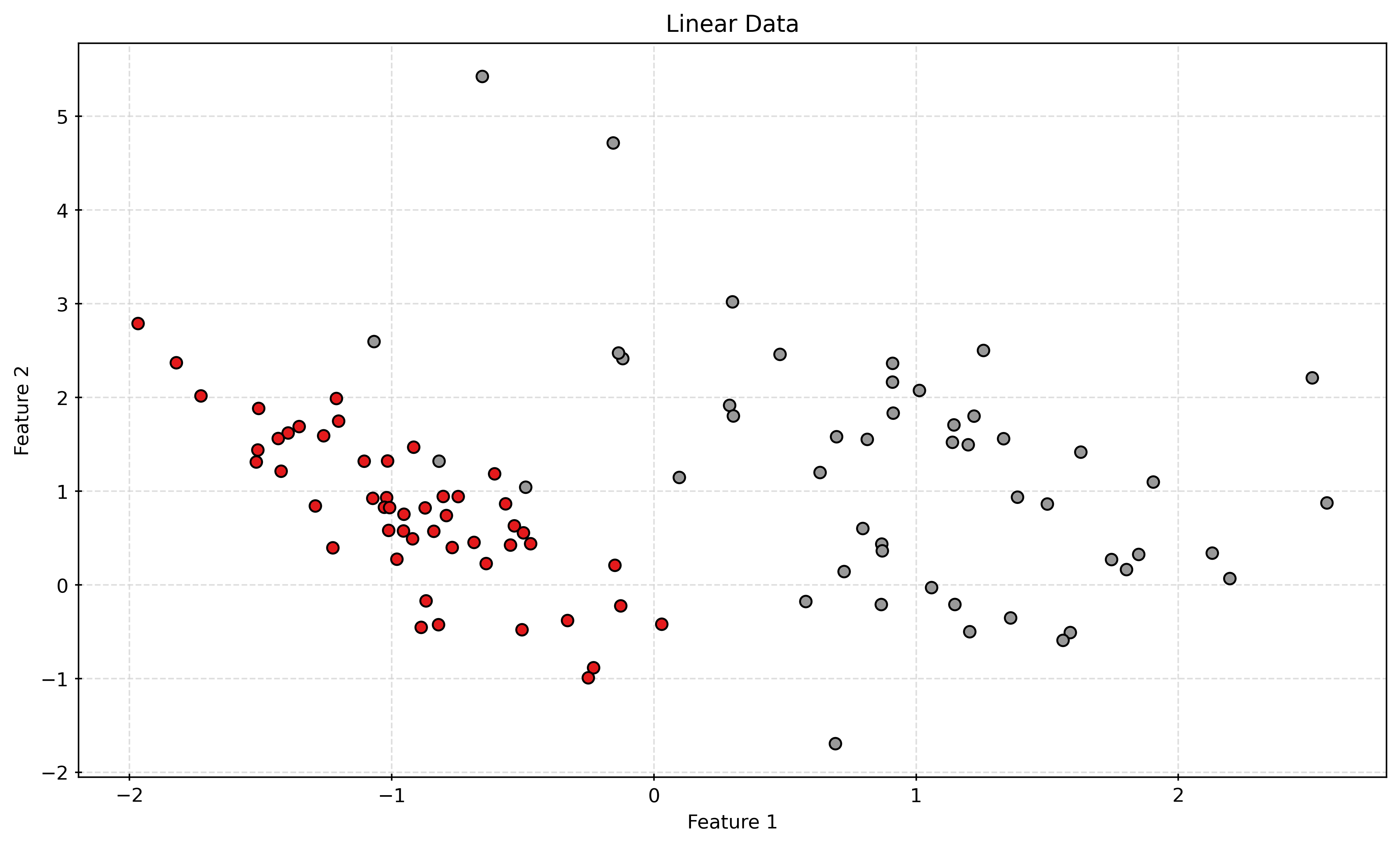

# define a logistic regression model class
class LogisticRegressionNN(nn.Module):
    def __init__(self, input_size):
        super().__init__()
        self.linear = nn.Linear(input_size, 1)
        self.sigmoid = nn.Sigmoid()

    def forward(self, x):
        out = self.linear(x)
        out = self.sigmoid(out)
        return out

# create the model instance
model = LogisticRegressionNN(X.shape[1])
print(model)

LogisticRegressionNN(
  (linear): Linear(in_features=2, out_features=1, bias=True)
  (sigmoid): Sigmoid()
)

# define the loss function
loss_fn = nn.BCELoss()
# loss_fn = nn.BCEWithLogitsLoss()

# define the optimizer
optimizer = torch.optim.Adam(
    model.parameters(),
    lr=0.01,
)

# convert the data to PyTorch tensors
X_tensor = torch.tensor(X, dtype=torch.float32)
y_tensor = torch.tensor(y, dtype=torch.float32)

# train the model
num_epochs = 1000
for epoch in range(num_epochs):

    # forward pass
    outputs = model(X_tensor)
    loss = loss_fn(outputs, y_tensor.view(-1, 1))

    # backward and optimize
    optimizer.zero_grad()
    loss.backward()
    optimizer.step()

# print the trained model parameters
print("Trained model parameters:")
for name, param in model.named_parameters():
    if param.requires_grad:
        print(name, param.data)

Trained model parameters:
linear.weight tensor([[3.7912, 1.6506]])
linear.bias tensor([-0.6449])

# fit sklearn logistic regression
sk_model = LogisticRegression(penalty=None)
_ = sk_model.fit(X, y)

# print the sklearn model parameters
sk_model.intercept_, sk_model.coef_

(array([1.07315953]), array([[15.06284414,  6.71249139]]))

# generate a grid of points
x_min, x_max = X[:, 0].min() - 1, X[:, 0].max() + 1
y_min, y_max = X[:, 1].min() - 1, X[:, 1].max() + 1
xx, yy = np.meshgrid(
    np.arange(x_min, x_max, 0.005),
    np.arange(y_min, y_max, 0.005),
)
grid_points = np.c_[xx.ravel(), yy.ravel()]

# convert the grid points to PyTorch tensor
grid_tensor = torch.tensor(grid_points, dtype=torch.float32)

# use the trained model to predict the class labels for the grid points
with torch.no_grad():
    predictions = model(grid_tensor)
    labels = (predictions >= 0.5).float().numpy().reshape(xx.shape)

# create a new figure and an axes
fig, ax = plt.subplots(figsize=(10, 6))

# plot the decision boundary
ax.contourf(xx, yy, labels, alpha=0.25, cmap=plt.cm.Set1)

# plot the generated data
scatter = ax.scatter(X[:, 0], X[:, 1], c=y, cmap=plt.cm.Set1)

# set labels and title
ax.set_xlabel("Feature 1")
ax.set_ylabel("Feature 2")
ax.set_title("Linear Data with Decision Boundary")

# add a legend
legend_elements = [
    plt.Line2D(
        [0],
        [0],
        marker="o",
        color="w",
        label="Class 0",
        markerfacecolor="grey",
        markersize=8,
    ),
    plt.Line2D(
        [0],
        [0],
        marker="o",
        color="w",
        label="Class 1",
        markerfacecolor="r",
        markersize=8,
    ),
]
ax.legend(handles=legend_elements)

# add a grid
ax.grid(color="lightgrey", linestyle="--")

# display the plot
plt.show()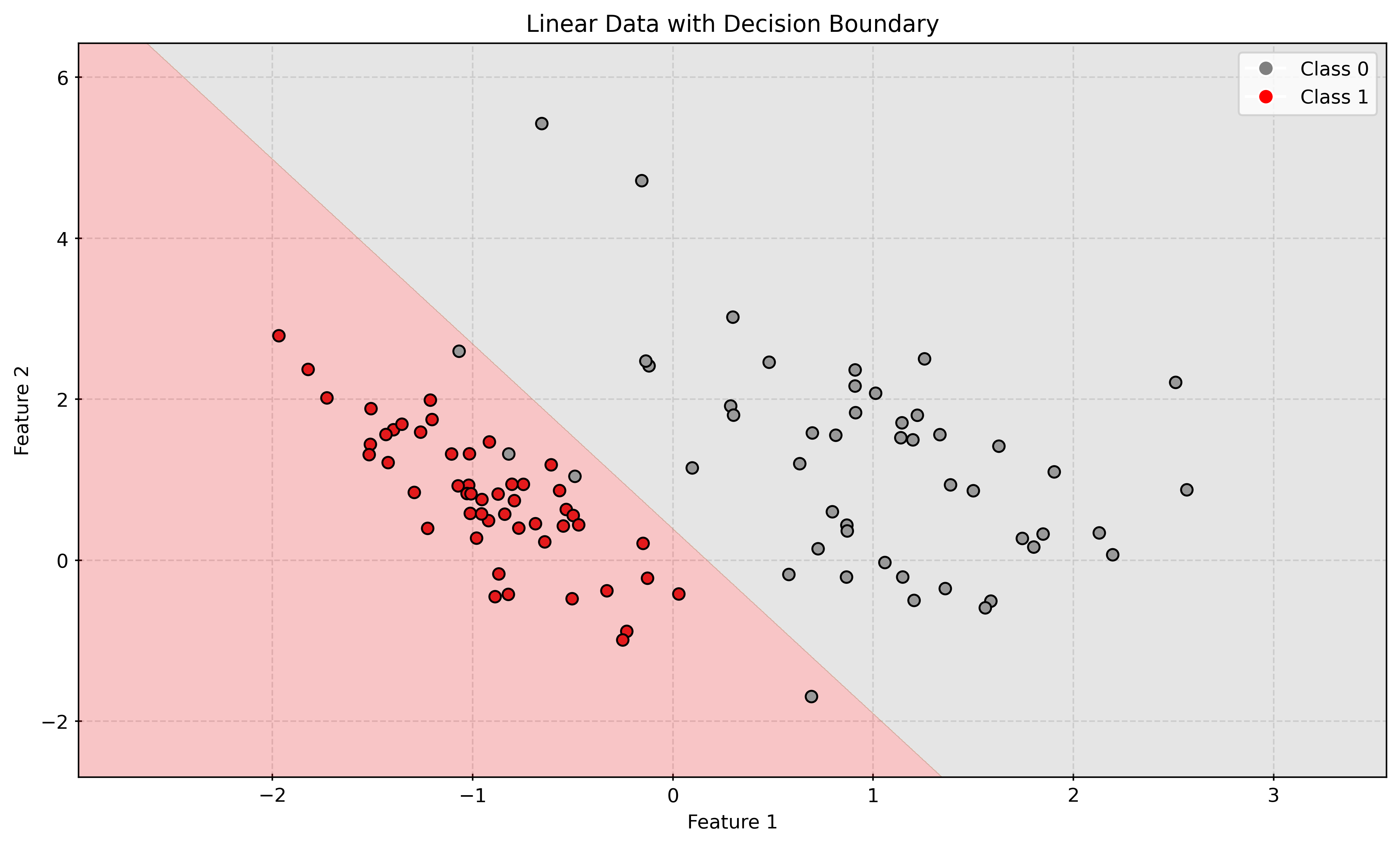

Logistic Regression as a Neural Network: Circle Data

# generate circles data
X, y = make_circles(
    n_samples=100,
    noise=0.05,
    random_state=42,
)

# plot the generated data
fig, ax = plt.subplots(figsize=(10, 6))
scatter = ax.scatter(
    X[:, 0],
    X[:, 1],
    c=y,
    cmap=plt.cm.Set1,
)
ax.set_xlabel("Feature 1")
ax.set_ylabel("Feature 2")
ax.set_title("Circles Data")
ax.grid(color="lightgrey", linestyle="--")
plt.show()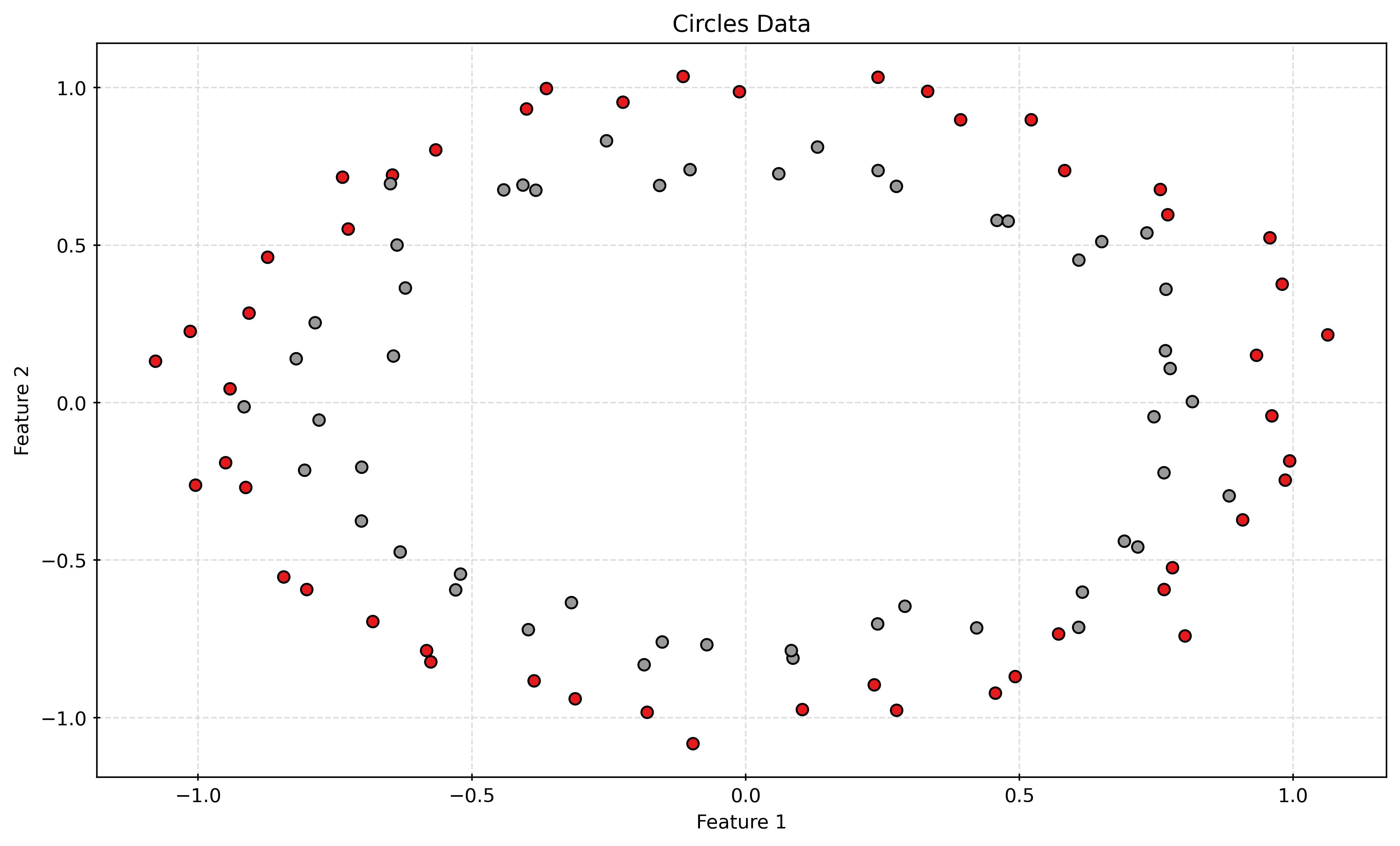

# create the model instance
model = LogisticRegressionNN(X.shape[1])
print(model)

# define the loss function
criterion = nn.BCELoss()

# define the optimizer
optimizer = torch.optim.Adam(
    model.parameters(),
    lr=0.01,
)

# convert the data to PyTorch tensors
X_tensor = torch.tensor(X, dtype=torch.float32)
y_tensor = torch.tensor(y, dtype=torch.float32)

# train the model
num_epochs = 1000
for epoch in range(num_epochs):

    # forward pass
    outputs = model(X_tensor)
    loss = criterion(outputs, y_tensor.view(-1, 1))

    # backward and optimize
    optimizer.zero_grad()
    loss.backward()
    optimizer.step()

LogisticRegressionNN(
  (linear): Linear(in_features=2, out_features=1, bias=True)
  (sigmoid): Sigmoid()
)

# print the trained model parameters
print("Trained model parameters:")
for name, param in model.named_parameters():
    if param.requires_grad:
        print(name, param.data)

Trained model parameters:
linear.weight tensor([[0.0180, 0.0113]])
linear.bias tensor([-2.0658e-05])

# generate a grid of points
x_min, x_max = X[:, 0].min() - 1, X[:, 0].max() + 1
y_min, y_max = X[:, 1].min() - 1, X[:, 1].max() + 1
xx, yy = np.meshgrid(
    np.arange(x_min, x_max, 0.005),
    np.arange(y_min, y_max, 0.005),
)
grid_points = np.c_[xx.ravel(), yy.ravel()]

# convert the grid points to PyTorch tensor
grid_tensor = torch.tensor(grid_points, dtype=torch.float32)

# use the trained model to predict the class labels for the grid points
with torch.no_grad():
    predictions = model(grid_tensor)
    labels = (predictions >= 0.5).float().numpy().reshape(xx.shape)

# create a new figure and an axes
fig, ax = plt.subplots(figsize=(10, 6))

# plot the decision boundary
ax.contourf(xx, yy, labels, alpha=0.5, cmap=plt.cm.Set1)

# plot the generated data
scatter = ax.scatter(X[:, 0], X[:, 1], c=y, cmap=plt.cm.Set1)

# set labels and title
ax.set_xlabel("Feature 1")
ax.set_ylabel("Feature 2")
ax.set_title("Linearly Separable Data with Decision Boundary")

# add a legend
legend_elements = [
    plt.Line2D(
        [0],
        [0],
        marker="o",
        color="w",
        label="Class 0",
        markerfacecolor="grey",
        markersize=8,
    ),
    plt.Line2D(
        [0],
        [0],
        marker="o",
        color="w",
        label="Class 1",
        markerfacecolor="r",
        markersize=8,
    ),
]
ax.legend(handles=legend_elements)

# add a grid
ax.grid(True, color="lightgrey")

# display the plot
plt.show()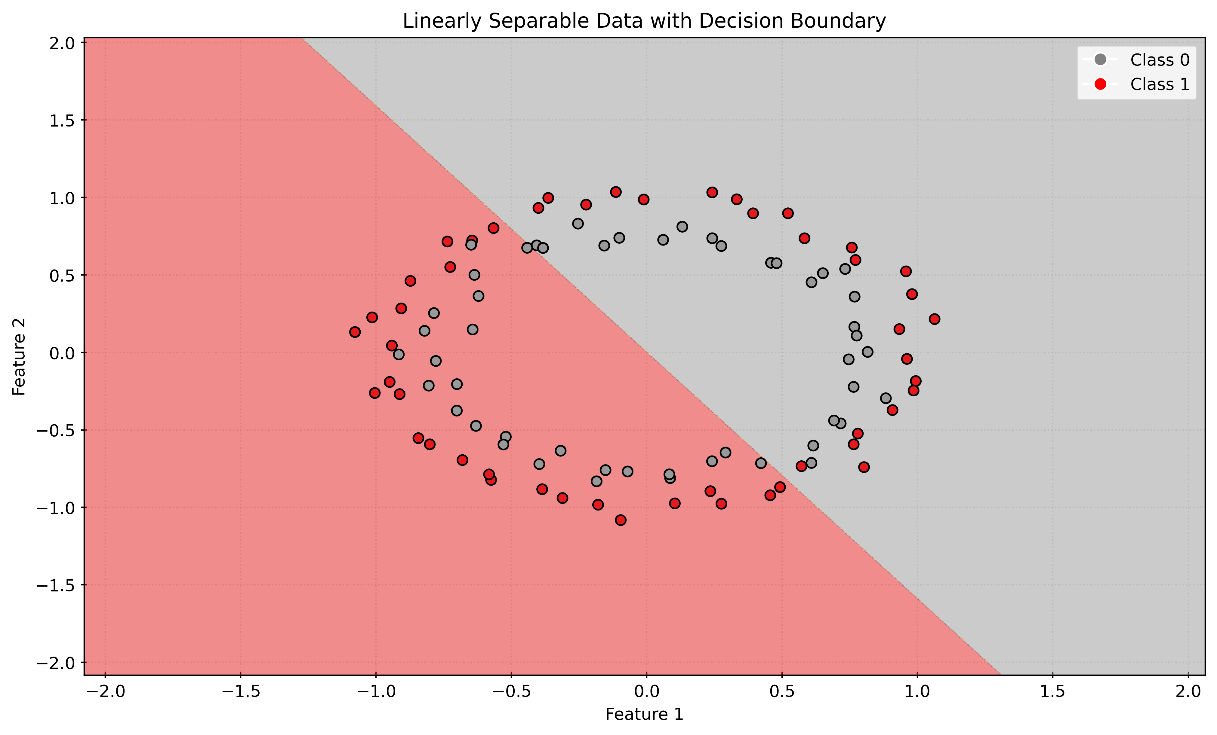

Multi-Layer Neural Network: Circle Data

# define multi-layer neural network class
class MLP(nn.Module):
    def __init__(self, input_size):
        super().__init__()
        self.linear = nn.Sequential(
            nn.Linear(input_size, 100),
            nn.ReLU(),
            nn.Linear(100, 10),
            nn.ReLU(),
            nn.Linear(10, 1),
        )
        self.sigmoid = nn.Sigmoid()

    def forward(self, x):
        out = self.linear(x)
        out = self.sigmoid(out)
        return out

# create the model instance
model = MLP(X.shape[1])
print(model)

# define the loss function
criterion = nn.BCELoss()

# define the optimizer
optimizer = torch.optim.SGD(
    model.parameters(),
    lr=0.1,
)

# convert the data to PyTorch tensors
X_tensor = torch.tensor(X, dtype=torch.float32)
y_tensor = torch.tensor(y, dtype=torch.float32)

# train the model
num_epochs = 1000
for epoch in range(num_epochs):
    # Forward pass
    outputs = model(X_tensor)
    loss = criterion(outputs, y_tensor.view(-1, 1))

    # Backward and optimize
    optimizer.zero_grad()
    loss.backward()
    optimizer.step()

MLP(
  (linear): Sequential(
    (0): Linear(in_features=2, out_features=100, bias=True)
    (1): ReLU()
    (2): Linear(in_features=100, out_features=10, bias=True)
    (3): ReLU()
    (4): Linear(in_features=10, out_features=1, bias=True)
  )
  (sigmoid): Sigmoid()
)

# print the trained model parameters
# print("Trained model parameters:")
# for name, param in model.named_parameters():
#     if param.requires_grad:
#         print(name, param.data)

# generate a grid of points
x_min, x_max = X[:, 0].min() - 1, X[:, 0].max() + 1
y_min, y_max = X[:, 1].min() - 1, X[:, 1].max() + 1
xx, yy = np.meshgrid(
    np.arange(x_min, x_max, 0.02),
    np.arange(y_min, y_max, 0.02),
)
grid_points = np.c_[xx.ravel(), yy.ravel()]

# convert the grid points to PyTorch tensor
grid_tensor = torch.tensor(grid_points, dtype=torch.float32)

# use the trained model to predict the class labels for the grid points
with torch.no_grad():
    predictions = model(grid_tensor)
    labels = (predictions >= 0.5).float().numpy().reshape(xx.shape)

# create a new figure and an axes
fig, ax = plt.subplots(figsize=(10, 6))

# plot the decision boundary
ax.contourf(xx, yy, labels, alpha=0.5, cmap=plt.cm.Set1)

# plot the generated data
scatter = ax.scatter(X[:, 0], X[:, 1], c=y, cmap=plt.cm.Set1)

# set labels and title
ax.set_xlabel("Feature 1")
ax.set_ylabel("Feature 2")
ax.set_title("Circle Data with Decision Boundary")

# add a legend
legend_elements = [
    plt.Line2D(
        [0],
        [0],
        marker="o",
        color="w",
        label="Class 0",
        markerfacecolor="grey",
        markersize=8,
    ),
    plt.Line2D(
        [0],
        [0],
        marker="o",
        color="w",
        label="Class 1",
        markerfacecolor="r",
        markersize=8,
    ),
]
ax.legend(handles=legend_elements)

# add a grid
ax.grid(True, color="lightgrey")

# display the plot
plt.show()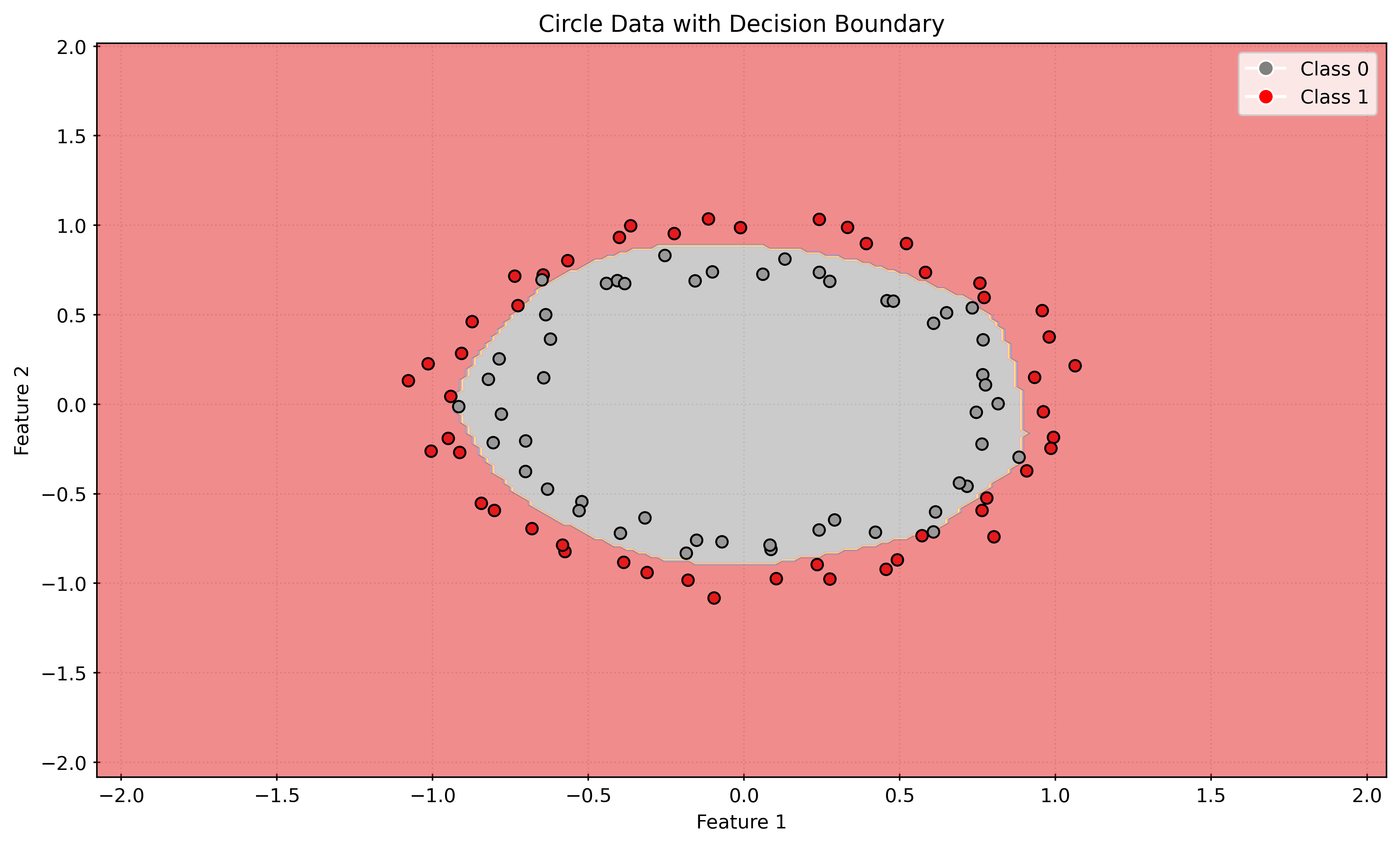

Multi-Layer Neural Network: Five Class Data

# generate the dataset
X, y = make_blobs(
    n_samples=1000,
    centers=5,
    random_state=42,
)

# print the shape of the dataset
print("Shape of X:", X.shape)
print("Shape of y:", y.shape)

Shape of X: (1000, 2)
Shape of y: (1000,)

# create a new figure and an axes
fig, ax = plt.subplots(figsize=(10, 6))

# plot the generated data
scatter = ax.scatter(
    X[:, 0],
    X[:, 1],
    c=y,
    cmap=plt.cm.Set1,
)

# set labels and title
ax.set_xlabel("Feature 1")
ax.set_ylabel("Feature 2")
ax.set_title("Linear Data")

# add a grid
ax.grid(color="lightgrey", linestyle="--")

# display the plot
plt.show()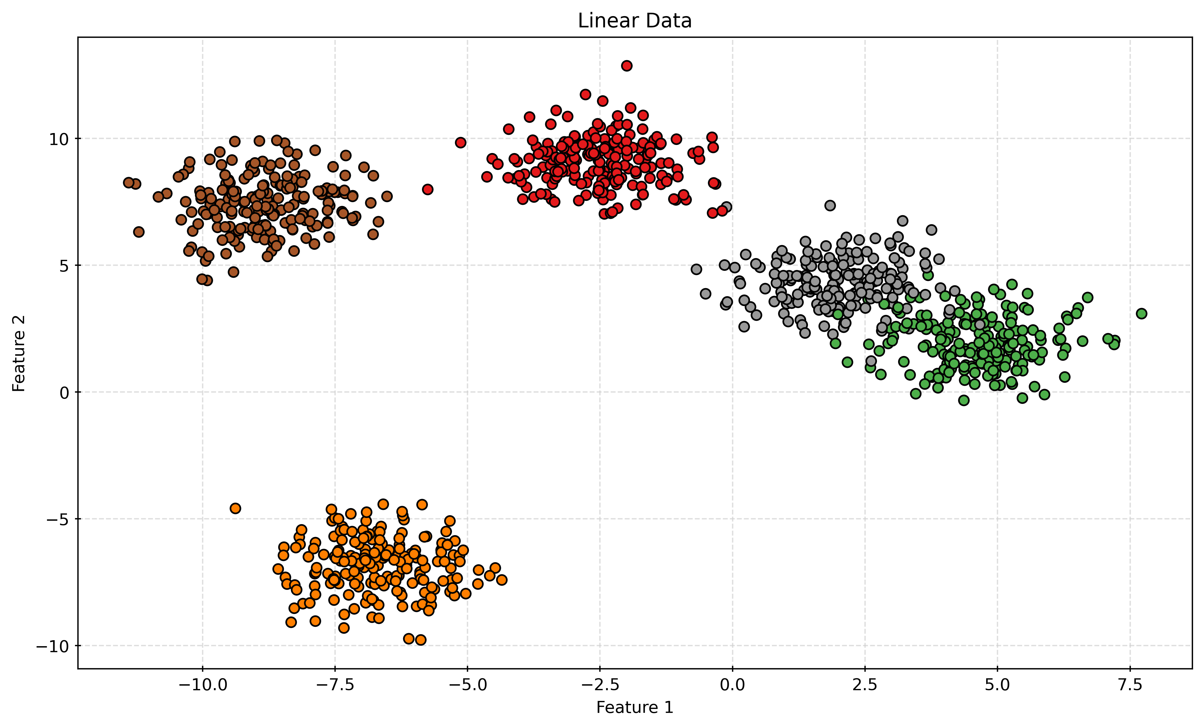

# check target data
y[:15]

array([1, 1, 2, 1, 4, 2, 3, 4, 1, 4, 4, 2, 3, 2, 3])

# define multi-layer neural network class
class MLP(nn.Module):
    def __init__(self, input_size):
        super().__init__()
        self.linear = nn.Sequential(
            nn.Linear(input_size, 100),
            nn.ReLU(),
            nn.Linear(100, 10),
            nn.ReLU(),
            nn.Linear(10, 10),
            nn.ReLU(),
            nn.Linear(10, 5),
        )

    def forward(self, x):
        out = self.linear(x)
        return out

# create the model instance
input_size = X.shape[1]
model = MLP(input_size)
print(model)

# define the loss function
criterion = nn.CrossEntropyLoss()

# define the optimizer
optimizer = torch.optim.Adam(
    model.parameters(),
    lr=0.01,
)

# convert the data to PyTorch tensors
X_tensor = torch.tensor(X, dtype=torch.float32)
y_tensor = torch.tensor(y, dtype=torch.long)

# train the model
num_epochs = 1000
for epoch in range(num_epochs):

    # forward pass
    outputs = model(X_tensor)
    loss = criterion(outputs, y_tensor)

    # backward and optimize
    optimizer.zero_grad()
    loss.backward()
    optimizer.step()

MLP(
  (linear): Sequential(
    (0): Linear(in_features=2, out_features=100, bias=True)
    (1): ReLU()
    (2): Linear(in_features=100, out_features=10, bias=True)
    (3): ReLU()
    (4): Linear(in_features=10, out_features=10, bias=True)
    (5): ReLU()
    (6): Linear(in_features=10, out_features=5, bias=True)
  )
)

# print the trained model parameters
# print("Trained model parameters:")
# for name, param in model.named_parameters():
#     if param.requires_grad:
#         print(name, param.data)

# convert the model predictions to numpy array
with torch.no_grad():
    predictions = model(X_tensor)
    predicted_labels = torch.argmax(predictions, dim=1).numpy()

# calculate the accuracy
accuracy = accuracy_score(y, predicted_labels)
print("Accuracy:", accuracy)

Accuracy: 0.98

# generate a grid of points
x_min, x_max = X[:, 0].min() - 1, X[:, 0].max() + 1
y_min, y_max = X[:, 1].min() - 1, X[:, 1].max() + 1
xx, yy = np.meshgrid(
    np.arange(x_min, x_max, 0.02),
    np.arange(y_min, y_max, 0.02),
)
grid_points = np.c_[
    xx.ravel(),
    yy.ravel(),
]

# convert the grid points to PyTorch tensor
grid_tensor = torch.tensor(grid_points, dtype=torch.float32)

# use the trained model to predict the class labels for the grid points
with torch.no_grad():
    predictions = model(grid_tensor)
    labels = torch.argmax(predictions, dim=1).numpy().reshape(xx.shape)

# create a new figure and an axes
fig, ax = plt.subplots(figsize=(10, 6))

# plot the decision boundary
ax.contourf(
    xx,
    yy,
    labels,
    alpha=0.5,
    cmap=plt.cm.Set1,
)

# plot the generated data
scatter = ax.scatter(
    X[:, 0],
    X[:, 1],
    c=y,
    cmap=plt.cm.Set1,
)

# set labels and title
ax.set_xlabel("Feature 1")
ax.set_ylabel("Feature 2")
ax.set_title("Decision Boundary")

# add a grid
ax.grid(True, color="lightgrey")

# display the plot
plt.show()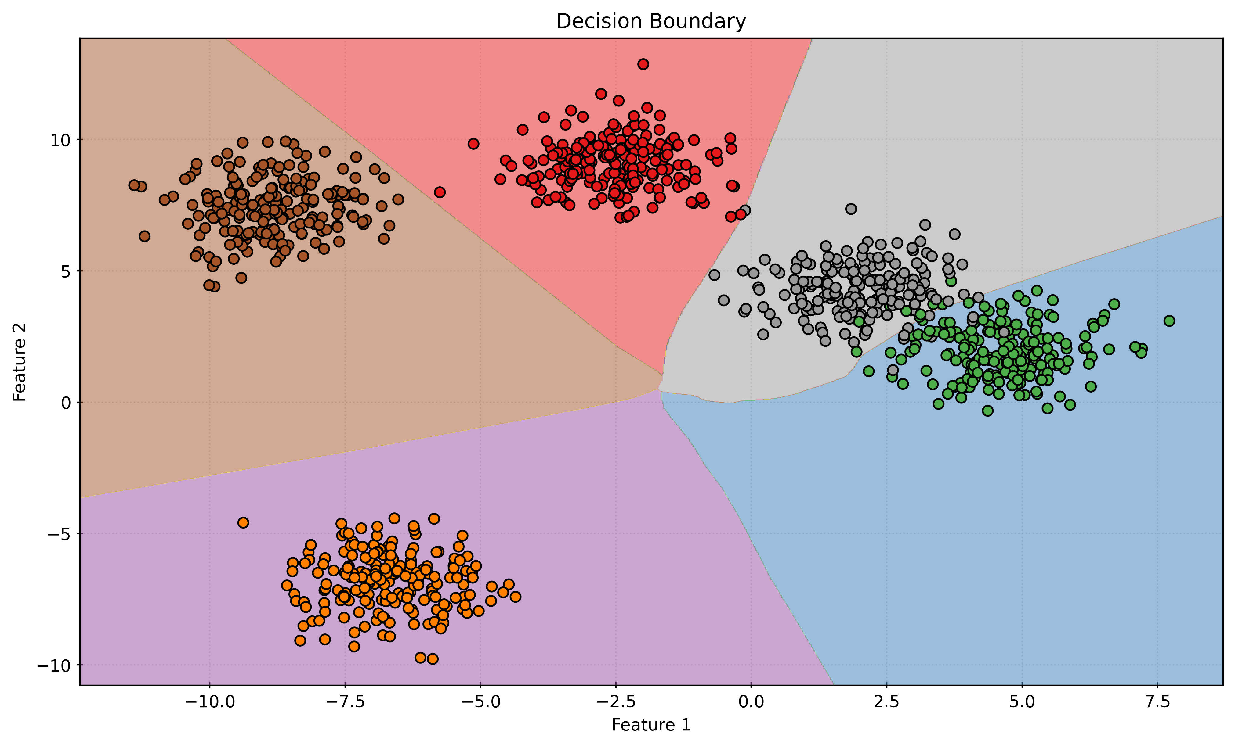

Convolutional Neural Networks

CNN Notebook

Additional Reading and Resources

• Deep Learning with PyTorch
• Learn PyTorch for Deep Learning: Zero to Mastery
  • Deep Learning Fundamentals: Slides | Notebook
  • Workflow Fundamentals: Slides | Notebook
  • Neural Networks for Classification: Slides | Notebook
  • Computer Vision: Slides | Notebook
• CNN Explainer
• CS231n: Deep Learning for Computer Vision
• Bishop: Deep Learning Foundations and Concepts
• Goodfellow: Deep Learning
• MIT 6.S191 Introduction to Deep Learning
• Prince: Understanding Deep Learning
• PyTorch Lightning
• Keras
• Wikipedia: Neural Networks
  • Wikipedia: Deep Learning
  • Wikipedia: Convolutional Neural Networks
  • Wikipedia: MNIST
  • Wikipedia: LeNet
  • Wikipedia: ImageNet
  • Wikipedia: AlexNet