# basics
import numpy as np
import pandas as pd
import seaborn as sns
import matplotlib.pyplot as plt

# machine learning
from sklearn.linear_model import LinearRegression
from sklearn.pipeline import Pipeline
from sklearn.preprocessing import PolynomialFeatures
from sklearn.preprocessing import FunctionTransformer
from sklearn.metrics import root_mean_squared_error
Linear Regression
The Classic Statistical Model
Setup and Objectives
In this note, we will discuss:
- using linear regression, specifically for regression tasks,
- parametric models, in contrast to non-parametric models,
- and the assumptions of the linear regression model.
Linear Regression Basics
To introduce linear regression, we’ll first demonstrate that the LinearRegression class in sklearn works like any other regressor.
# helper function to simulate data for regression task
def sim_reg_data(n=25, seed=42):
    np.random.seed(seed)
    x1 = np.random.uniform(low=0, high=5, size=(n,))
    x2 = np.random.uniform(low=4, high=7, size=(n,))
    x1 = np.round(x1, 2)
    x2 = np.round(x2, 2)
    e = np.random.normal(loc=0, scale=1, size=n)
    y = 2 + 3 * x1 + 0.5 * x2 + e
    y = np.round(y, 2)
    X = np.column_stack((x1, x2))
    return X, y
The function above simulates some data for a regression task. Specifically, it creates a target y that is a linear combination of two features x1 and x2, plus some noise. More specifically, we assume:
\[ Y = 2 + 3x_1 + 0.5x_2 + \epsilon. \]
Later, we will consider this the “true” model.
# simulate a train and test set
X_train, y_train = sim_reg_data(
    n=200,
    seed=42,
)
X_test, y_test = sim_reg_data(
    n=100,
    seed=307,
)
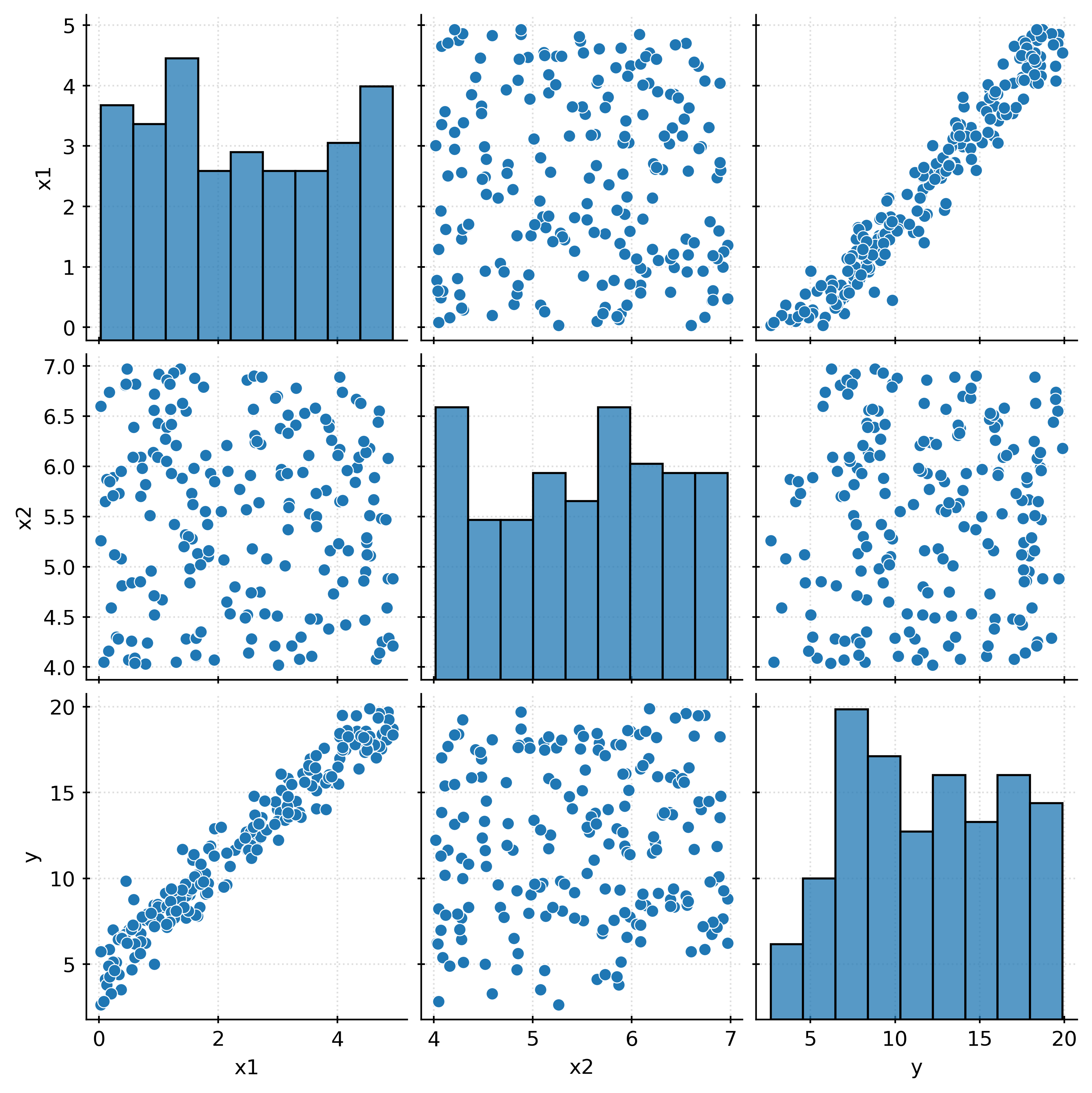
After simulating some train and test data, we briefly inspect the data.
# temporarily create df for easy plotting and nice printing
train_df = pd.DataFrame(
    {
        "x1": X_train[:, 0],
        "x2": X_train[:, 1],
        "y": y_train,
    }
)
train_df| x1 | x2 | y | |
|---|---|---|---|
| 0 | 1.87 | 5.93 | 11.88 |
| 1 | 4.75 | 4.25 | 18.40 |
| 2 | 3.66 | 4.48 | 15.90 |
| 3 | 2.99 | 6.70 | 14.01 |
| 4 | 0.78 | 5.82 | 7.57 |
| ... | ... | ... | ... |
| 195 | 1.75 | 6.79 | 9.81 |
| 196 | 3.63 | 6.58 | 16.45 |
| 197 | 4.49 | 5.29 | 18.06 |
| 198 | 4.44 | 6.25 | 18.21 |
| 199 | 3.90 | 6.26 | 15.92 |
200 rows × 3 columns
The above “pairs” plot, shows all pairwise relationships between the available variables, both the target and the features.
With the data simulated and inspected, we can now fit a linear regression model to the data.
# instantiate a liner regression
lr = LinearRegression()

# fit linear regression to the train data
_ = lr.fit(X_train, y_train)

# make prediction for first five observations of the test set
lr.predict(X_test[:5])
array([ 9.74686651, 11.38944255, 11.10014178, 18.41619462, 16.27374679])Here, we’ve done the usual steps for a regression task:
- Instantiate the regressor object.
- Fit the regressor to data.
- Make predictions on some data.
Notably, the LinearRegression class has very few parameters. While there are some parameters, we will not modify them, and thus there are effectively zero tuning parameters for this model.
How does linear regression work? First, recall the usual setup for the regression task. We have a target \(Y\) and features \(x\), and we want to learn a function \(f\), the signal, that maps \(x\) to \(Y\). However, don’t forget that the target \(Y\) is also impacted by noise, \(\epsilon\).
\[ Y = f(x) + \epsilon \]
Linear regression assumes that the signal is a linear combination of the features.
\[ Y = \beta_0 + \beta_1 x_1 + \beta_2 x_2 + \ldots + \beta_p x_p + \epsilon \]
That is, linear regression assumes:
\[ f(x) = \beta_0 + \beta_1 x_1 + \beta_2 x_2 + \ldots + \beta_p x_p. \]
In the brief example above, we specifically assumed:
\[ f(x) = \beta_0 + \beta_1 x_1 + \beta_2 x_2 \]
When we fit the model, we learned (estimated) the coefficients \(\beta_0\), \(\beta_1\), and \(\beta_2\).
# access the learned (estimated) coefficients
lr.intercept_, lr.coef_
(2.3227373410822256, array([3.00223949, 0.43968892]))- \(\hat{\beta}_0 = 2.323\)
- \(\hat{\beta}_1 = 3.002\)
- \(\hat{\beta}_2 = 0.44\)
Because this data was simulated, we can compare the learned coefficients to the true coefficients.
- \(\beta_0 = 2\)
- \(\beta_1 = 3\)
- \(\beta_2 = 0.5\)
The learned coefficients are “close” to the true coefficients, but of course not exactly the same, given the noisy relationship. In statistics, much thought would be given to the uncertainty in the learned coefficients. However, in machine learning, we instead focus on evaluating the model’s predictive performance.
To make predictions, we simply use the learned coefficients in place of the unknown coefficients.
\[ \hat{f}(x) = \hat{\beta}_0 + \hat{\beta}_1 x_1 + \hat{\beta}_2 x_2 \]
In general, the learned function is:
\[ \hat{f}(x) = \hat{\beta}_0 + \hat{\beta}_1 x_1 + \hat{\beta}_2 x_2 + \ldots + \hat{\beta}_p x_p \]
Fitting Linear Regression
So, how are the coefficients learned? The usual method is to minimize the residual sum of squares (RSS).1
\[ \text{RSS}(\beta_0, \beta_1, \beta_2, \ldots, \beta_p) = \sum_{i = 1}^{n}(y_i - (\beta_0 + \beta_1 x_{i1} + \beta_2 x_{i2} + \ldots + \beta_p x_{ip}))^2 \]
Note that the RSS is a function of the coefficients.
We find the coefficients that minimize the sum of the squared differences between the observed target and the predicted target. Given data \((\pmb{x}_i, y_i)\), we want to find the coefficients \(\beta_0, \beta_1, \beta_2, \ldots, \beta_p\) that minimize the the residual sum of squares.
\[ \underset{\beta_0, \beta_1, \beta_2, \ldots, \beta_p}{\text{min}} \sum_{i = 1}^{n}(y_i - (\beta_0 + \beta_1 x_{i1} + \beta_2 x_{i2} + \ldots + \beta_p x_{ip}))^2 \]
From here, we can use calculus to find the minimum, first taking a derivative with respect to each coefficient.2
Matrix Form
Instead of working with the summation above, and taking a derivative with respect to each coefficient, we can instead rewrite the problem in matrix form.
\[ X = \begin{bmatrix} 1 & x_{11} & x_{12} & \ldots & x_{1p} \\ 1 & x_{21} & x_{22} & \ldots & x_{2p} \\ \vdots & \vdots & \vdots & \ddots & \vdots \\ 1 & x_{n1} & x_{n2} & \ldots & x_{np} \\ \end{bmatrix} \]
\[ \beta = \begin{bmatrix} \beta_0 \\ \beta_1 \\ \beta_2 \\ \vdots \\ \beta_p \\ \end{bmatrix} \]
\[ \epsilon = \begin{bmatrix} \epsilon_1 \\ \epsilon_2 \\ \vdots \\ \epsilon_n \\ \end{bmatrix} \]
\[ y = \begin{bmatrix} y_1 \\ y_2 \\ \vdots \\ y_n \\ \end{bmatrix} \]
\[ y = X \beta + \epsilon \]
Derivation of \(\hat{\beta}\)
To derive the ordinary least squares (OLS) estimator \(\hat{\beta}\), we start with the linear regression model in matrix form as shown above.
\[ y = X \beta + \epsilon \]
where:
- \(Y\) is an \(n \times 1\) vector of observed values,
- \(X\) is an \(n \times (p+1)\) matrix of predictors (including a column of ones for the intercept),
- \(\beta\) is a \((p+1) \times 1\) vector of unknown coefficients,
- \(\epsilon\) is an \(n \times 1\) vector of errors.
The goal is to find \(\hat{\beta}\) that minimizes the sum of squared residuals, which is now written in matrix form as:
\[ \text{RSS} = (y - X\beta)^T (y - X\beta) \]
To find the minimum, we take the derivative of the RSS with respect to \(\beta\) and set it to zero:
\[ \frac{\partial \text{RSS}}{\partial \beta} = -2X^T(y - X\beta) = 0 \]
Solving for \(\beta\), we get:
\[ X^T Y = X^T X \beta \]
Assuming \(X^T X\) is invertible, we can solve for \(\beta\):
\[ \hat{\beta} = (X^T X)^{-1} X^T y \]
To make predictions, we simply substitute \(\hat{\beta}\) into the model:
\[ \hat{y} = X \hat{\beta} \]
Parametric Models
Linear regression, like logistic regression, is a parametric model. This means that the model makes assumptions about the form of the relationship between the features and the target, as a function of parameters to be learned. In the case of linear regression, the model assumes that the relationship is linear, specifically a linear combination of the features. This assumption is often not realistic, because it is too simple. But that simplification has some advantages that are useful in some situations.
Linear Model Assumptions
For the purposes of machine learning, we focus on the assumption that the target is a linear combination of the features. However, more broadly, the usual linear regression model makes several additional assumptions.
Technically, the assumptions are mostly revealed by the model specification.
\[ Y = \beta_0 + \beta_1 x_1 + \beta_2 x_2 + \ldots + \beta_p x_p + \epsilon \]
\[ \epsilon \sim N(0, \sigma^2) \]
Note that now we have added an assumption about the error term \(\epsilon\).
We could instead write:
\[ Y \mid X = x \sim N(\beta_0 + \beta_1 x_1 + \beta_2 x_2 + \ldots + \beta_p x_p, \sigma^2) \]
When asked “What are the assumptions of linear regression?”, the following list is often given:
- Linearity: The target is a linear combination of the features, plus an error term.
- Independence: The errors are independent.
- Normality: The errors are normally distributed.
- Equal Variance: The errors have constant variance.
There are some additional more implicit assumptions:
- No perfect multicollinearity: No feature is a linear combination of the other features.
- Fixed \(x\): The features are fixed, not random.
- More samples than features: There are more samples than features.
While these assumptions are good to know, they are not necessary in a machine learning context. These assumptions are necessary for the usual statistical inference that is done with linear regression, for example, hypothesis tests and confidence intervals about the coefficients.
\[ H_0: \beta_1 = 0 \]
Without these assumptions, the usual test statistics and confidence intervals are not valid. As we are not using these tests, we can ignore these assumptions. While we would like for the linearity assumption to be met, we will not directly check the assumption and instead validate linear models as we would any other model.
Linear Model Flexibility
Although linear models have no tuning parameters, we can still manipulate their flexibility. If we consider a linear model that uses all available features to be the most flexible, we can reduce the flexibility by removing features. If we have available features \(x_1, x_2, x_3, \ldots, x_p\), we can fit a model using only a subset of the features.
Consider two models:
Model 1
\[ Y = \beta_0 + \beta_1 x_1 + \beta_2 x_2 + \epsilon \]
Model 2
\[ Y = \beta_0 + \beta_1 x_1 + \beta_2 x_2 + \beta_3 x_3 + \ldots + \beta_p x_p + \epsilon \]
Here, the first model is of course less flexible than the second model. Because the second model contains all of the features included in the first model, and more, we say that the first model is a nested model of the second model. In general, a model is nested within another model if the set of features in the first model is a subset of the set of features in the second model. A nest model is less flexible than the model in which it is nested.
Note that we cannot compare the flexibility of two models that are not nested. For example, we cannot compare the flexibility of the following two models:
Model 1
\[ Y = \beta_0 + \beta_1 x_1 + \beta_2 x_2+ \epsilon \]
Model 2
\[ Y = \beta_0 + \beta_1 x_1 + \beta_3 x_3 + \epsilon \]
In this case, the two models are not nested, and thus we cannot say that one is more flexible than the other.
As always, the flexibility of a model is related to the bias-variance tradeoff. So far, we’ve seen that using more features increases the flexibility of a model. However, note that so long as a linear model includes all necessary features, it is unbiased, that is its bias is 0. Of course we can only make this determination if we know the “true” model.
Consider the following true model:
\[ Y = 2 + 3 x_1 + 0.5 x_2 + 5 x_3 + \epsilon \]
Fitting any linear model that includes all three features will be unbiased.
For example, both of the following models are unbiased:
Model 1
\[ Y = \beta_0 + \beta_1 x_1 + \beta_2 x_2 + \beta_3 x_3 + \epsilon \]
Model 2
\[ Y = \beta_0 + \beta_1 x_1 + \beta_2 x_2+ \beta_3 x_3 + \beta_4 x_4 + \beta_5 x_5 + \epsilon \]
While both models are unbiased, the second model is more flexible than the first model, and thus is more variable.
Of course if we consider a model that does not include all necessary features, then the model will be biased.
Model 3
\[ Y = \beta_0 + \beta_1 x_1 + \epsilon \]
Because it does not include all of the relevant features, Model 3 is biased. It cannot capture the true relationship between the features and the target.
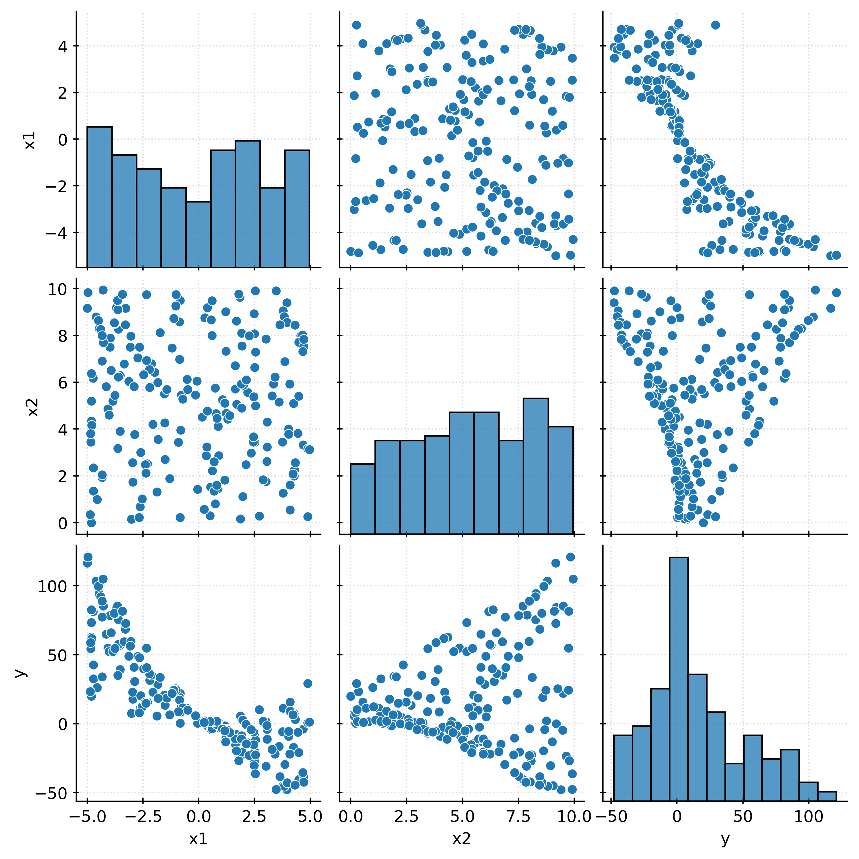
Higher Order Terms
# function to simulate data for regression task
def sim_reg_data_higher(n=25, seed=42):
    np.random.seed(seed)
    x1 = np.random.uniform(low=-5, high=5, size=(n,))
    x2 = np.random.uniform(low=0, high=10, size=(n,))
    x1 = np.round(x1, 2)
    x2 = np.round(x2, 2)
    e = np.random.normal(loc=0, scale=1, size=n)
    y = 1 + 1 * x1 + 0.5 * x2 + (x1**2) - 2 * (x1 * x2) + e
    y = np.round(y, 2)
    X = np.column_stack((x1, x2))
    return X, y
# simulate a train and test set
X_train, y_train = sim_reg_data_higher(
n=200,
seed=1,
)
X_test, y_test = sim_reg_data_higher(
n=100,
seed=2,
)# temporarily create df for easy plotting and nice printing
train_df = pd.DataFrame(
{
"x1": X_train[:, 0],
"x2": X_train[:, 1],
"y": y_train,
}
)
train_df| x1 | x2 | y | |
|---|---|---|---|
| 0 | -0.83 | 9.50 | 22.03 |
| 1 | 2.20 | 5.57 | -13.73 |
| 2 | -5.00 | 9.16 | 116.45 |
| 3 | -1.98 | 6.42 | 30.71 |
| 4 | -3.53 | 3.90 | 39.28 |
| ... | ... | ... | ... |
| 195 | 4.32 | 8.44 | -44.52 |
| 196 | -4.86 | 3.81 | 58.87 |
| 197 | -2.66 | 7.50 | 47.90 |
| 198 | 1.17 | 5.11 | -5.17 |
| 199 | 4.49 | 5.41 | -20.98 |
200 rows × 3 columns
# learn "polynomial" features (all second-order terms and below, without intercept)
poly = PolynomialFeatures(degree=2, include_bias=False)
_ = poly.fit(X_train)
Here we temporarily note the feature names for the original data, and then check the order of the created features.
# temporarily define feature names for original X data
poly.feature_names_in_ = ["x1", "x2"]

# check order of created features
# note that the interaction appears between the two quadratic terms
poly.get_feature_names_out()
array(['x1', 'x2', 'x1^2', 'x1 x2', 'x2^2'], dtype=object)Importantly, notice that the interaction term appears between the two quadratic terms.
Before proceeding, we remove the temporary feature names as they would interfere with the pipeline.
# remove temporary feature names
poly.feature_names_in_ = None
# preview the transformation
poly.transform(X_train[:5])array([[ -0.83 , 9.5 , 0.6889, -7.885 , 90.25 ],
[ 2.2 , 5.57 , 4.84 , 12.254 , 31.0249],
[ -5. , 9.16 , 25. , -45.8 , 83.9056],
[ -1.98 , 6.42 , 3.9204, -12.7116, 41.2164],
[ -3.53 , 3.9 , 12.4609, -13.767 , 15.21 ]])# initialize a first-order linear regression
lr_first = LinearRegression()
# create a pipeline with polynomial features and linear regression
lr_second = Pipeline(
[
("poly", PolynomialFeatures(degree=2, include_bias=False)),
("lr", LinearRegression()),
]
)
# fit both models
_ = lr_first.fit(X_train, y_train)
_ = lr_second.fit(X_train, y_train)# access the learned (estimated) coefficients
lr_first.intercept_, lr_first.coef_(8.087601042282472, array([-10.0721793 , 1.13117992]))# access the learned (estimated) coefficients
lr_second.named_steps['lr'].intercept_, lr_second.named_steps['lr'].coef_(0.7155757335097075,
array([ 0.98203002, 0.61993987, 1.00488342, -1.99189121, -0.01133566]))train_rmse_first = root_mean_squared_error(
y_train,
lr_first.predict(X_train),
)
train_rmse_second = root_mean_squared_error(
y_train,
lr_second.predict(X_train),
)
print(f"(First-Order Model) Train RMSE: {train_rmse_first:.3f}")
print(f"(Second-Order Model) Train RMSE: {train_rmse_second:.3f}")(First-Order Model) Train RMSE: 19.251
(Second-Order Model) Train RMSE: 1.005test_rmse_first = root_mean_squared_error(y_test, lr_first.predict(X_test),)
test_rmse_second = root_mean_squared_error(y_test, lr_second.predict(X_test),)
print(f"(First-Order Model) Test RMSE: {test_rmse_first:.3f}")
print(f"(Second-Order Model) Train RMSE: {test_rmse_second:.3f}")(First-Order Model) Test RMSE: 17.524
(Second-Order Model) Train RMSE: 1.042Feature Transformation
In addition to adding higher-order terms, we can also apply any arbitrary transformation to any feature. Doing so can provide the flexibility needed to allow a linear model to capture a wider variety of non-linear relationships.
Recall the sine wave example that we have seen several times.
def simulate_sin_data(n=25, sd=0.25, seed=42):
    np.random.seed(seed)
    X = np.random.uniform(low=-2 * np.pi, high=2 * np.pi, size=(n, 1))
    signal = np.sin(X).ravel()
    noise = np.random.normal(loc=0, scale=sd, size=n)
    y = signal + noise
    return X, y
# simulate a train and test set
X_train, y_train = simulate_sin_data(
n=200,
seed=42,
)
X_test, y_test = simulate_sin_data(
n=100,
seed=307,
)# fit a linear regression without any transformation
lr_standard = LinearRegression()
_ = lr_standard.fit(X_train, y_train)test_rmse_standard = root_mean_squared_error(
y_test,
lr_standard.predict(X_test),
)
print(f"(No Transformation) Test RMSE: {test_rmse_standard:.3f}")(No Transformation) Test RMSE: 0.695# plot learned regression (without transformed features)
x_plot = np.linspace(-2 * np.pi, 2 * np.pi, 1000).reshape((1000, 1))
fig, ax = plt.subplots()
ax.scatter(X_train, y_train, label="Actual")
ax.plot(x_plot, lr_standard.predict(x_plot), color="red", label="Fitted")
ax.set_xlabel("X_train")
ax.set_ylabel("y")
ax.set_ylim(-3, 3)
ax.grid(color="lightgrey", linestyle="--")
ax.legend()
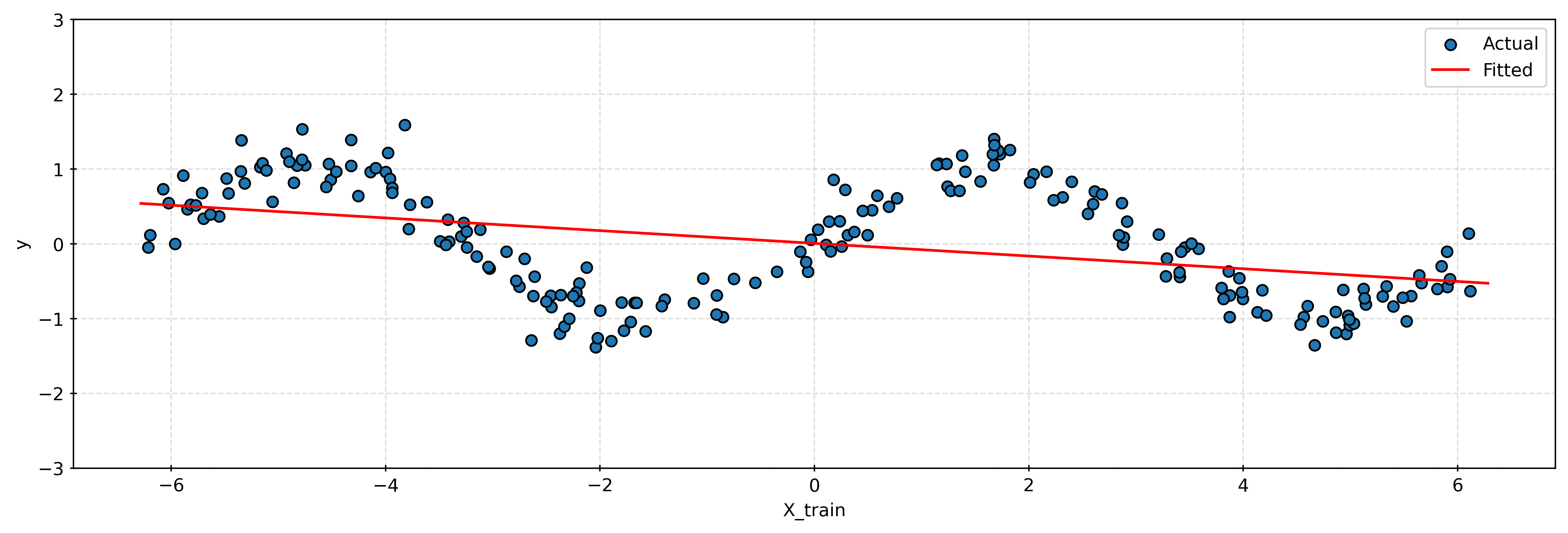
plt.show()Using a linear model without any transformation, we clearly see that the model is unable to capture the sine wave pattern.
# create a pipeline with the custom transformer and linear regression
lr_transformed = Pipeline(
    [
        ("sin_transformer", FunctionTransformer(np.sin)),
        ("lr", LinearRegression()),
    ]
)

# fit the pipeline to the training data
_ = lr_transformed.fit(X_train, y_train)
test_rmse_transformed = root_mean_squared_error(
y_test,
lr_transformed.predict(X_test),
)
print(f"(With Transformation) Test RMSE: {test_rmse_transformed:.3f}")(With Transformation) Test RMSE: 0.239# plot learned regression (without transformed features)
x_plot = np.linspace(-2 * np.pi, 2 * np.pi, 1000).reshape((1000, 1))
fig, ax = plt.subplots()
ax.scatter(X_train, y_train, label="Actual")
ax.plot(x_plot, lr_transformed.predict(x_plot), color="red", label="Fitted")
ax.set_xlabel("X_train")
ax.set_ylabel("y")
ax.set_ylim(-3, 3)
ax.grid(color="lightgrey", linestyle="--")
ax.legend()
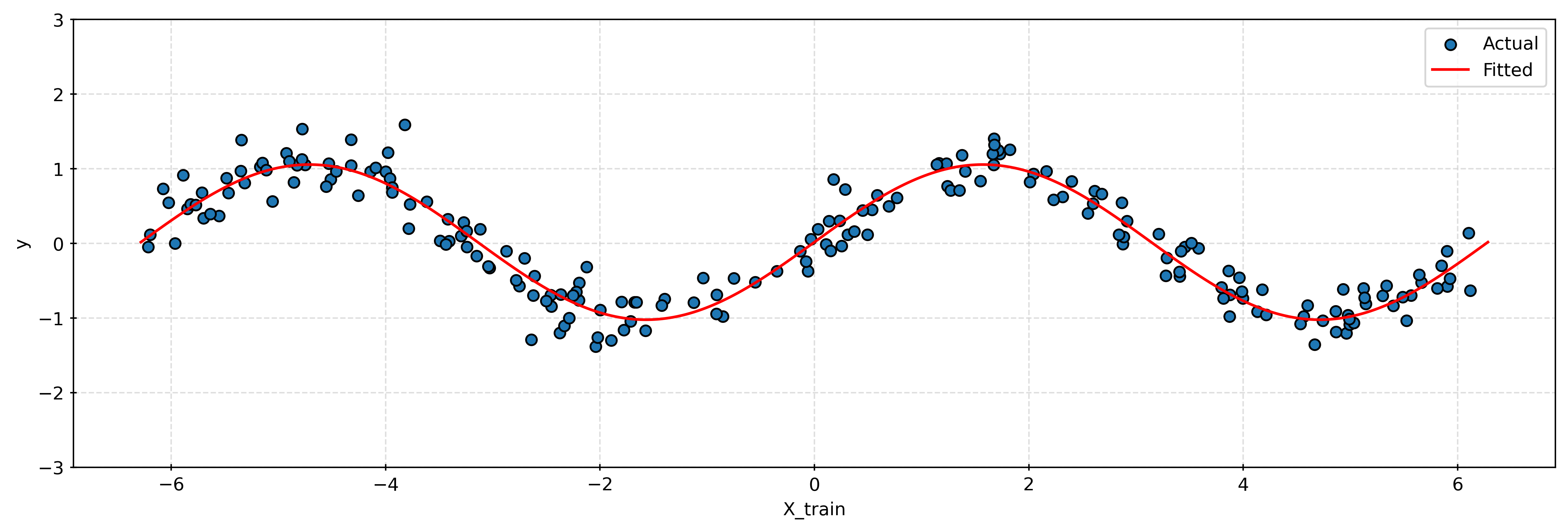
plt.show()While linear models can be improved by transforming the features, in practice it will rarely be so obvious which transformation to apply. If a linear model is not sufficient, it will often be more effective to try a nonparametric model that will more readily be able to learn complicated relationships.


