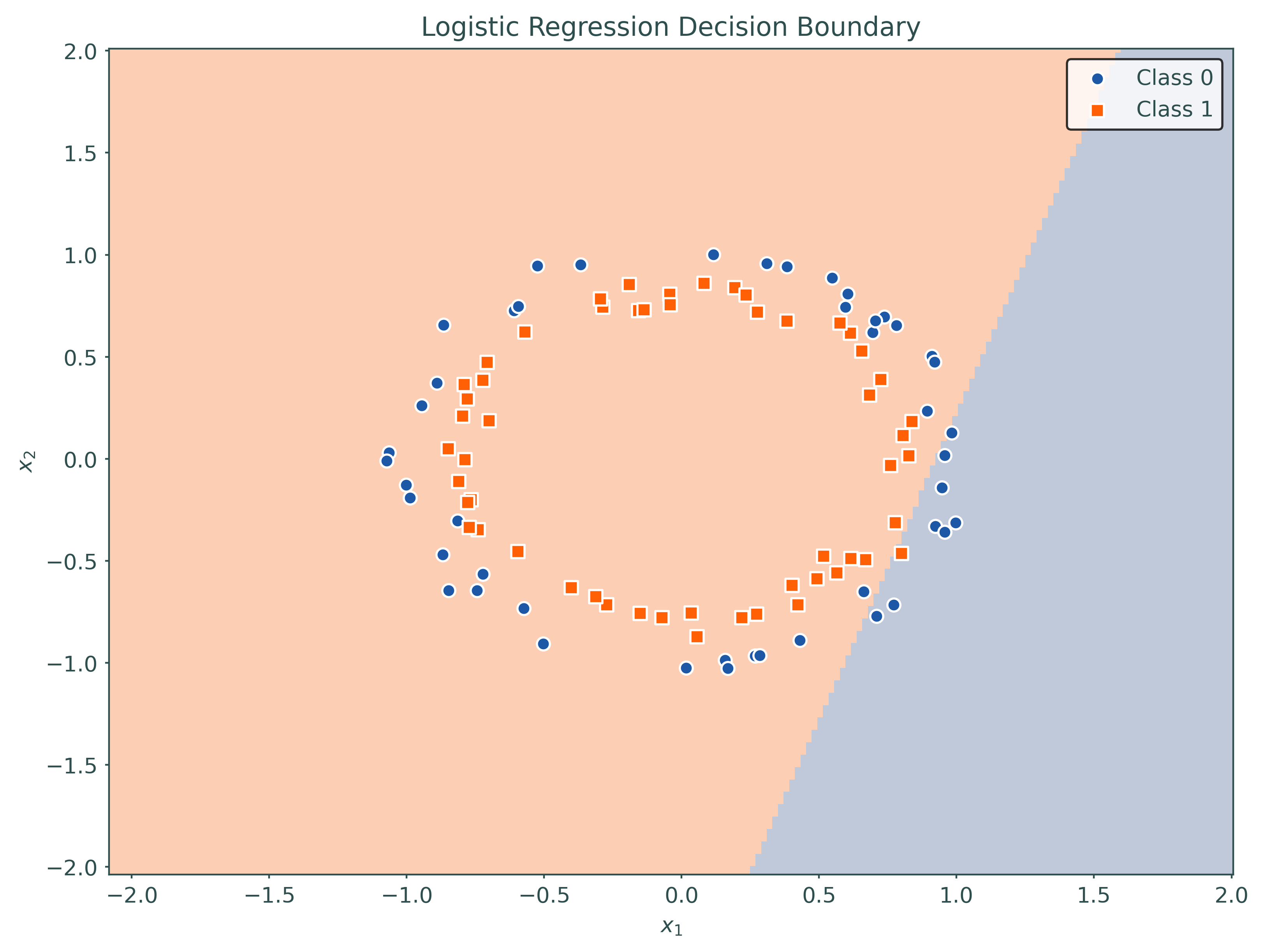
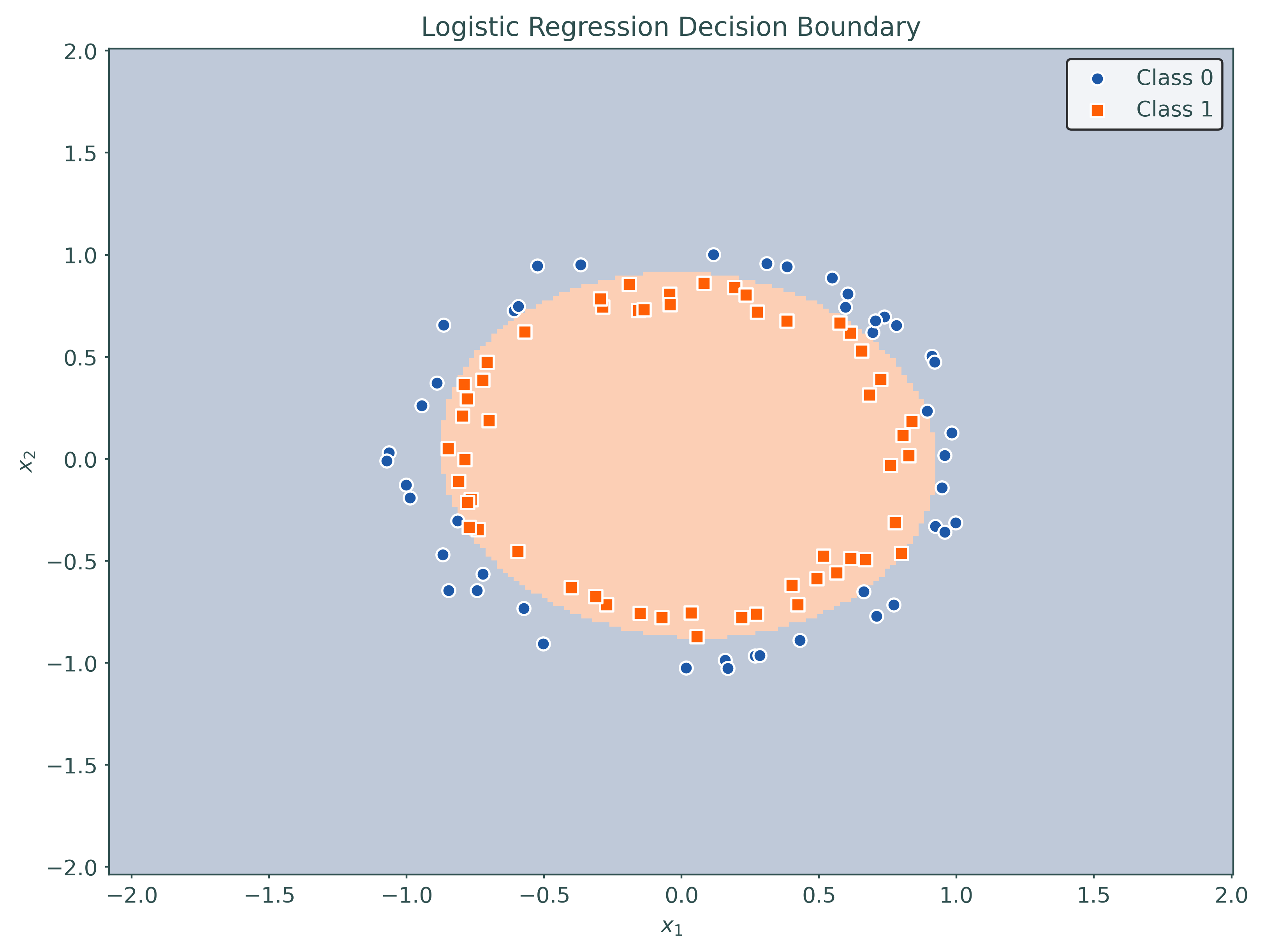
# basics
import numpy as np
import pandas as pd
import seaborn as sns
import matplotlib.pyplot as plt
from matplotlib.colors import ListedColormap

# machine learning
from sklearn.datasets import make_blobs, make_circles
from sklearn.pipeline import Pipeline
from sklearn.preprocessing import PolynomialFeatures
from sklearn.linear_model import LogisticRegression
from sklearn.model_selection import train_test_split
from sklearn.inspection import DecisionBoundaryDisplay
from sklearn.metrics import accuracy_scoreLogistic Regression
A Parametric Classification Model
Binary Classification Setup
Logistic regression is a model for a binary target. Recall that in a binary setting, we often encode the target as \(Y \in \{0, 1\}\). Because we are mostly concerned with \(P[Y = 1 \mid \pmb{X} = \pmb{x}]\), we define a useful shorthand notation.
\[ p(\pmb{x}) = P[Y = 1 \mid \pmb{X} = \pmb{x}] \]
\[ P[Y = 0 \mid \pmb{X} = \pmb{x}] + P[Y = 1 \mid \pmb{X} = \pmb{x}] = 1 \]
\[ 1 - p(\pmb{x}) = P[Y = 0 \mid \pmb{X} = \pmb{x}] \]
Logistic Regression Model
\[ \log\left(\frac{p(\pmb{x})}{1 - p(\pmb{x})}\right) = \beta_0 + \beta_1 x_1 + \ldots + \beta_p x_p \]
\[ \frac{p(\pmb{x})}{1 - p(\pmb{x})} = \frac{P[Y = 1 \mid \pmb{X} = \pmb{x}]}{P[Y = 0 \mid \pmb{X} = \pmb{x}]} \]
\[ p(\pmb{x}) = P[Y = 1 \mid \pmb{X} = \pmb{x}] = \frac{e^{\beta_0 + \beta_1 x_{1} + \cdots + \beta_p x_p}}{1 + e^{\beta_0 + \beta_1 x_{1} + \cdots + \beta_p x_p}} \]
\[ \text{logit}(\xi) = \log\left(\frac{\xi}{1 - \xi}\right) \]
\[ \sigma(\xi) = \text{logit}^{-1}(\xi) = \frac{e^\xi}{1 + e^{\xi}} = \frac{1}{1 + e^{-\xi}} \]
\[ \eta(\pmb{x}) = \beta_0 + \beta_1 x_1 + \ldots + \beta_p x_p \]
\[ \log\left(\frac{p(\pmb{x})}{1 - p(\pmb{x})}\right) = \eta(\pmb{x}) \]
\[ p(\pmb{x}) = \sigma(\eta(\pmb{x})) = \frac{e^{\eta(\pmb{x})}}{1 + e^{\eta(\pmb{x})}} = \frac{1}{1 + e^{-\eta(\pmb{x})}} = \frac{1}{1 + e^{-(\beta_0 + \beta_1 x_1 + \ldots + \beta_p x_p)}} \]
\[ Y \mid \pmb{X} = \pmb{x} \sim \text{Bernoulli}(p(\pmb{x})) \]
Examples in Python
# helper function to convert numpy (two column) X and y to a pandas df
# useful for printing and plotting
def numpy_to_df(X, y):
    df = pd.DataFrame(
        {
            "x1": X[:, 0],
            "x2": X[:, 1],
            "y": y,
        }
    )
    return df
# helper function to create a custom decision region plot
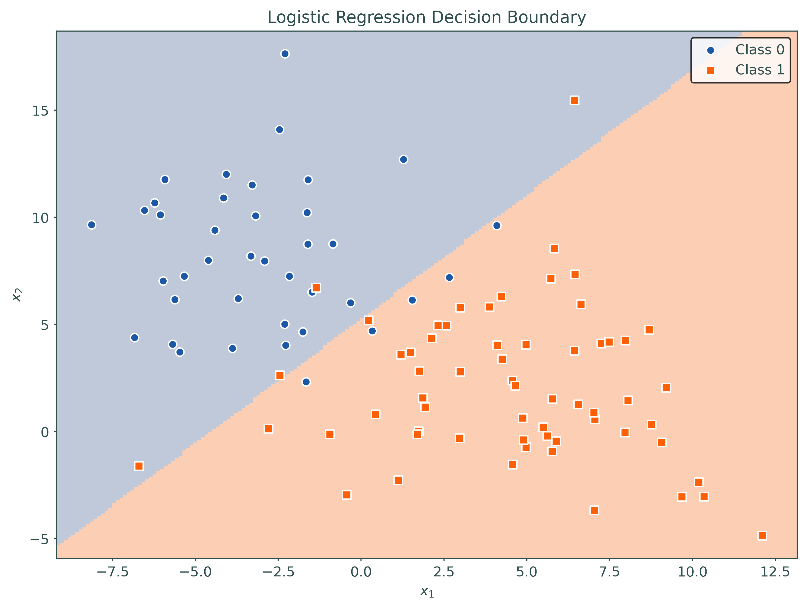
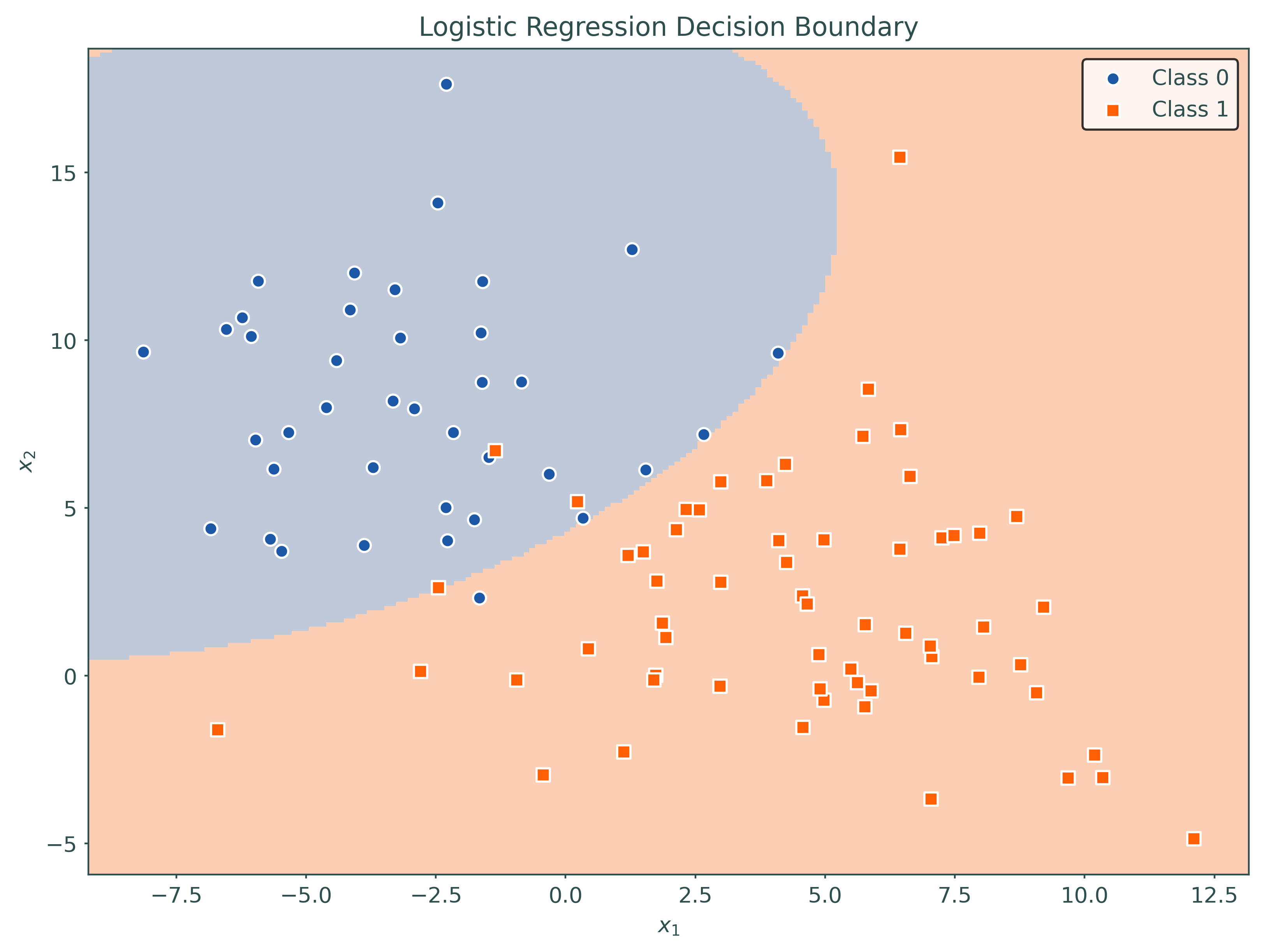
def plot_decision_regions(mod, X, y):
# define colors for points
illini_cmap = ListedColormap(
[
"#1D58A7", # illini industrial blue
"#FF5F05", # illini orange
]
)
# define colors for decision regions
light_illini_cmap = ListedColormap(
[
"#BFC9D9", # illini industrial blue (lighter)
"#FCCFB5", # a lighter orange
]
)
# create figure and axes
_, ax = plt.subplots(figsize=(8, 6))
# start with sklearn default plot
DecisionBoundaryDisplay.from_estimator(
mod,
X,
cmap=light_illini_cmap,
ax=ax,
grid_resolution=200,
response_method="predict",
plot_method="pcolormesh",
shading="auto",
xlabel="$x_1$",
ylabel="$x_2$",
)
# add points to plot
for i, shape in enumerate(["o", "s"]):
mask = y == i
ax.scatter(
X[mask, 0],
X[mask, 1],
color=illini_cmap(i),
edgecolors="white",
linewidth=1,
marker=shape,
label=f"Class {i}",
)
# add title and legend
_ = ax.set_title("Logistic Regression Decision Boundary")
_ = ax.legend(loc="best")
# show plot
plt.show()# make "blob" data for classification
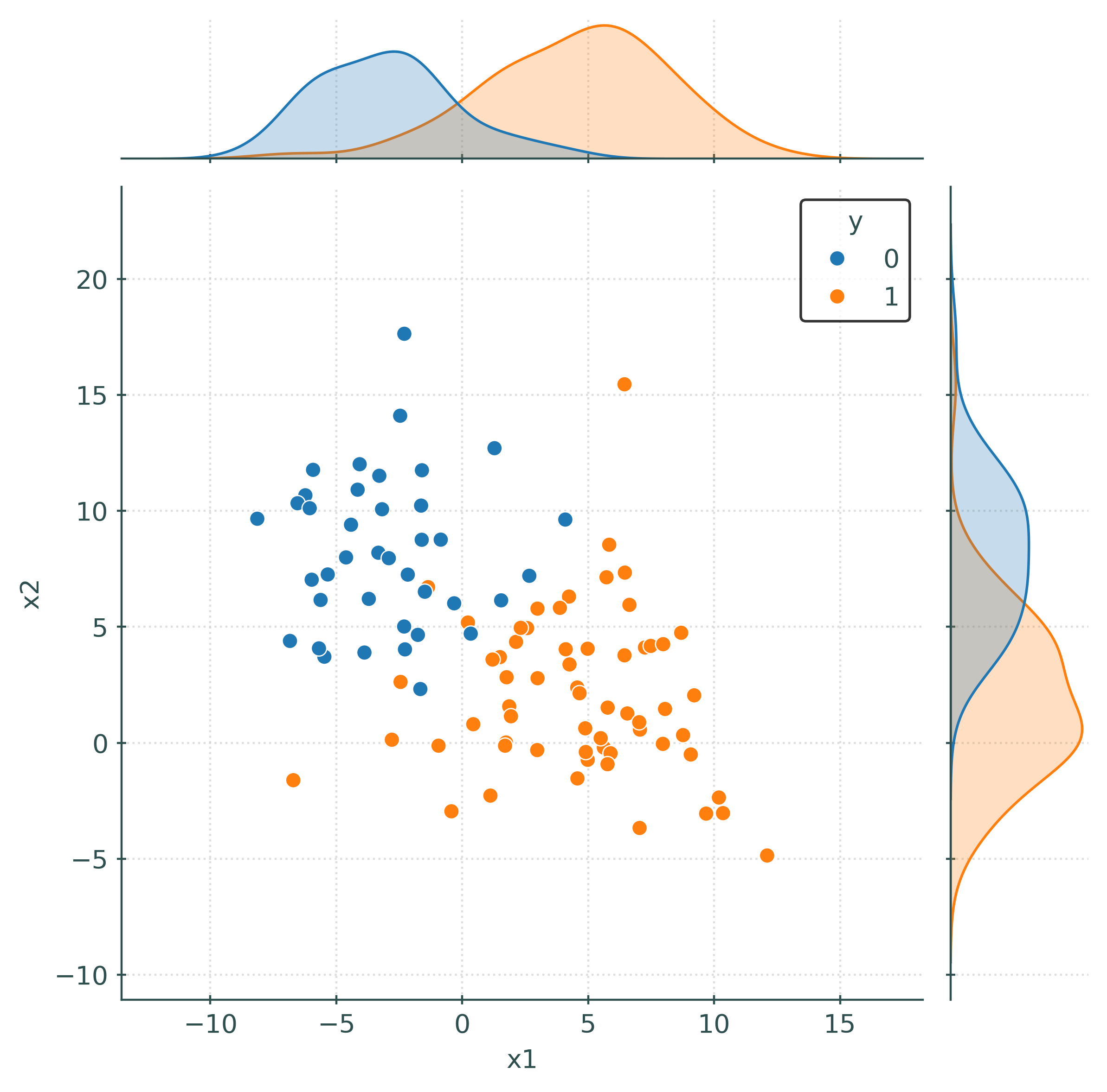
X, y = make_blobs(
n_samples=200,
centers=2,
cluster_std=3.5,
random_state=42,
)
# split the "blob" data
X_train, X_test, y_train, y_test = train_test_split(
X,
y,
test_size=0.50,
random_state=42,
)
# temporarily create df for easy plotting and printing
train_df = numpy_to_df(X_train, y_train)
train_df| x1 | x2 | y | |
|---|---|---|---|
| 0 | 5.62 | -0.21 | 1 |
| 1 | -5.98 | 7.03 | 0 |
| 2 | -5.62 | 6.16 | 0 |
| 3 | -0.43 | -2.95 | 1 |
| 4 | -8.14 | 9.66 | 0 |
| ... | ... | ... | ... |
| 95 | 7.98 | 4.25 | 1 |
| 96 | -6.70 | -1.61 | 1 |
| 97 | -3.18 | 10.07 | 0 |
| 98 | 2.32 | 4.96 | 1 |
| 99 | 12.11 | -4.86 | 1 |
100 rows × 3 columns
# (quickly) create a "joint" plot
_ = sns.jointplot(data=train_df, x="x1", y="x2", hue="y")
plt.show()# initialize and fit logistic regression
logistic = LogisticRegression(penalty=None)
_ = logistic.fit(X_train, y_train)
# estimated coefficients
logistic.intercept_, logistic.coef_(array([3.63406579]), array([[ 0.80226887, -0.69174668]]))# estimated conditional probabilities (first 10 samples from test set)
np.round(logistic.predict_proba(X_test)[range(10)], 3)array([[0.982, 0.018],
[0.628, 0.372],
[1. , 0. ],
[0.992, 0.008],
[1. , 0. ],
[0.798, 0.202],
[0.35 , 0.65 ],
[0. , 1. ],
[1. , 0. ],
[0.012, 0.988]])# predictions (classifications) on the test data
logistic.predict(X_test)array([0, 0, 0, 0, 0, 0, 1, 1, 0, 1, 0, 0, 0, 0, 0, 1, 0, 1, 1, 0, 0, 1,
0, 0, 0, 1, 1, 1, 1, 1, 1, 1, 1, 0, 0, 0, 1, 1, 0, 0, 0, 0, 0, 0,
1, 0, 0, 1, 1, 0, 1, 1, 1, 0, 0, 0, 1, 0, 0, 0, 0, 1, 1, 1, 1, 1,
1, 0, 0, 0, 0, 0, 1, 1, 0, 0, 1, 0, 0, 0, 1, 1, 0, 0, 0, 1, 1, 0,
1, 1, 1, 0, 0, 0, 1, 0, 0, 1, 1, 0])# train accuracy
accuracy_score(y_train, logistic.predict(X_train))
# test accuracy
accuracy_score(y_test, logistic.predict(X_test))0.92# create "second order" features (without bias/intercept, it will be "added" later)
poly = PolynomialFeatures(degree=2, include_bias=False)
# "learn" the transformation then apply it to the train and test data
_ = poly.fit(X_train)
X_train_trans = poly.transform(X_train)
X_test_trans = poly.transform(X_test)
# initialize and fit logistic regression with higher order terms
logistic_higher = LogisticRegression(penalty=None)
_ = logistic_higher.fit(X_train_trans, y_train)
# estimated coefficients
logistic_higher.intercept_, logistic_higher.coef_(array([6.73899122]),
array([[ 1.22657355, -1.90522748, 0.06187221, -0.0475074 , 0.07781114]]))# train accuracy
accuracy_score(y_train, logistic_higher.predict(X_train_trans))0.96# test accuracy
accuracy_score(y_test, logistic_higher.predict(X_test_trans))0.94# refit the higher-order model using a pipeline
# # this is helpful for plotting decision boundary, also better in practice
pipeline = Pipeline(
[
("poly", PolynomialFeatures(degree=2, include_bias=False)),
("logistic", LogisticRegression(penalty=None)),
]
)
pipeline.fit(X_train, y_train)Pipeline(steps=[('poly', PolynomialFeatures(include_bias=False)),
('logistic', LogisticRegression(penalty=None))])In a Jupyter environment, please rerun this cell to show the HTML representation or trust the notebook. On GitHub, the HTML representation is unable to render, please try loading this page with nbviewer.org.
Pipeline(steps=[('poly', PolynomialFeatures(include_bias=False)),
('logistic', LogisticRegression(penalty=None))])PolynomialFeatures(include_bias=False)
LogisticRegression(penalty=None)
# make and split "circle" data for classification
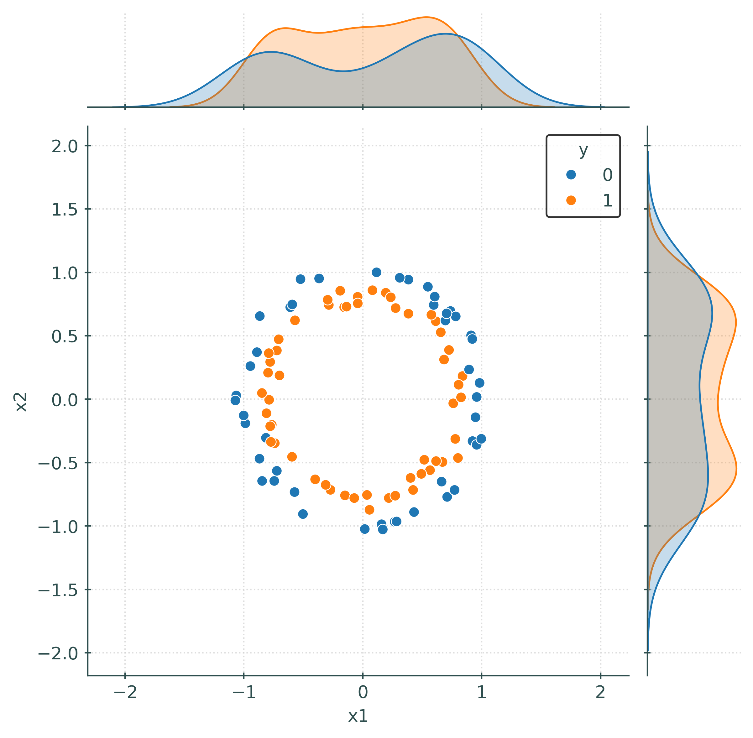
X, y = make_circles(
n_samples=200,
random_state=42,
noise=0.05,
)
X_train, X_test, y_train, y_test = train_test_split(
X,
y,
test_size=0.50,
random_state=42,
)# temporarily create df for easy plotting
train_df = numpy_to_df(X_train, y_train)
train_df| x1 | x2 | y | |
|---|---|---|---|
| 0 | -0.19 | 0.86 | 1 |
| 1 | -0.81 | -0.30 | 0 |
| 2 | 0.40 | -0.62 | 1 |
| 3 | -0.52 | 0.95 | 0 |
| 4 | -0.80 | 0.21 | 1 |
| ... | ... | ... | ... |
| 95 | 0.70 | 0.68 | 0 |
| 96 | 0.49 | -0.59 | 1 |
| 97 | 0.83 | 0.01 | 1 |
| 98 | 0.80 | -0.46 | 1 |
| 99 | -0.79 | 0.36 | 1 |
100 rows × 3 columns
# (quickly) create a "joint" plot
_ = sns.jointplot(data=train_df, x="x1", y="x2", hue="y")# initialize and fit logistic regression
logistic = LogisticRegression(penalty=None)
_ = logistic.fit(X_train, y_train)
# plot decision region for initial model
plot_decision_regions(logistic, X_train, y_train)
# setup a higher-order model using a pipeline
pipeline = Pipeline(
[
("poly", PolynomialFeatures(degree=2, include_bias=False)),
("logistic", LogisticRegression(penalty=None)),
]
)
# fit a higher-order model using a pipeline
pipeline.fit(X_train, y_train)Pipeline(steps=[('poly', PolynomialFeatures(include_bias=False)),
('logistic', LogisticRegression(penalty=None))])In a Jupyter environment, please rerun this cell to show the HTML representation or trust the notebook. On GitHub, the HTML representation is unable to render, please try loading this page with nbviewer.org.
Pipeline(steps=[('poly', PolynomialFeatures(include_bias=False)),
('logistic', LogisticRegression(penalty=None))])PolynomialFeatures(include_bias=False)
LogisticRegression(penalty=None)
Footnotes
This is likely true for computer scientists as well, but they also have good reason to use base 2 logarithms.↩︎
