# basic imports
import numpy as np
import pandas as pd
import seaborn as sns
import matplotlib.pyplot as plt

# model imports
from sklearn.neighbors import KNeighborsRegressor
from sklearn.neighbors import KNeighborsClassifier

# metric imports
from sklearn.metrics import root_mean_squared_error
from sklearn.metrics import accuracy_score

# model selection imports
from sklearn.model_selection import train_test_split
from sklearn.model_selection import KFold
from sklearn.model_selection import cross_val_score
from sklearn.model_selection import GridSearchCV

# preprocessing imports
from sklearn.preprocessing import StandardScaler
from sklearn.preprocessing import OneHotEncoder
from sklearn.impute import SimpleImputer
from sklearn.compose import make_column_transformer
from sklearn.pipeline import make_pipeline

# data imports
from sklearn.datasets import make_friedman1Generalization
Model Flexibility, Overfitting, and the Bias-Variance Tradeoff
Setup and Objectives
Model Flexibility
A model’s flexibility determines how well the model can learn the training data.
- A “flexible” model can learn “complex” patterns in the data, but is also more likely to overfit.
- An “inflexible” model is less likely to overfit, but may not be able to learn the true underlying patterns in the data.
Given a particular dataset, when fitting a model, you are essentially trying to find a model that is flexible enough to learn the underlying patterns in the data, but not so flexible that it learns the noise in the data.
How do we control a model’s flexibility? Our main tool for controlling a model’s flexibility is the available hyperparameters (tuning parameters).
Let’s investigate with \(k\) for \(k\)-nearest neighbors.
# simulate data
X, y = make_friedman1(
    n_samples=1000,
    noise=0.25,
    random_state=42,
)
# split the data
X_train, X_test, y_train, y_test = train_test_split(
X,
y,
test_size=0.25,
random_state=42,
)# define range of k values to search over
k_values = range(1, 152, 2)# initialize storage for train RMSE values
train_rmse = []
# initialize storage for test RMSE values
test_rmse = []# fit models and calculate train and test test RMSE for each value of k
for k in k_values:
# initialize model, with the current k
knn = KNeighborsRegressor(n_neighbors=k)
# fit the model to the (validation) train data
knn.fit(X_train, y_train)
# get train predictions
y_train_pred = knn.predict(X_train)
# calculate (and store) train RMSE
train_rmse.append(root_mean_squared_error(y_train, y_train_pred))
# get test predictions
y_test_pred = knn.predict(X_test)
# calculate (and store) test RMSE
test_rmse.append(root_mean_squared_error(y_test, y_test_pred))# plot RMSE against k
fig, ax = plt.subplots(figsize=(10, 6))
ax.plot(k_values, train_rmse, marker="o", markersize=5, label="Train RMSE")
ax.plot(k_values, test_rmse, marker="o", markersize=5, label="Test RMSE")
ax.set_xlabel("k")
ax.set_ylabel("RMSE")
ax.set_title("k versus Error")
ax.legend()
plt.show()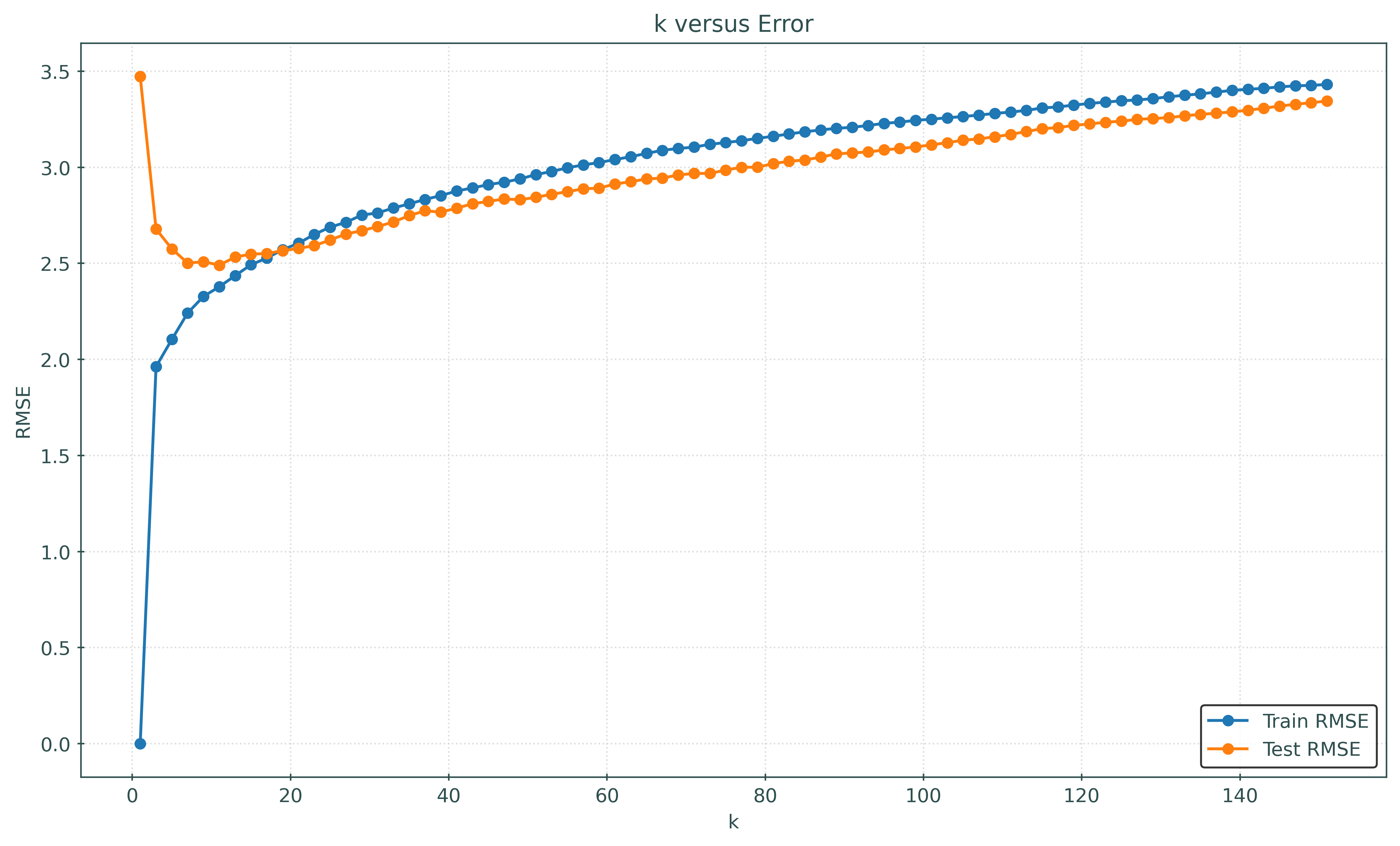
How does \(k\) relate to model flexibility?
- A small \(k\) has low train error, thus is more flexible model.
- A large \(k\) has high train error, thus is a less flexible model.
That is, as \(k\) increases, the model becomes less flexible.
How do we know this? Note that as \(k\) increases, the train RMSE increases. Said in reverse, as \(k\) decreases, the train RMSE decreases, and thus the model better learns the training data.
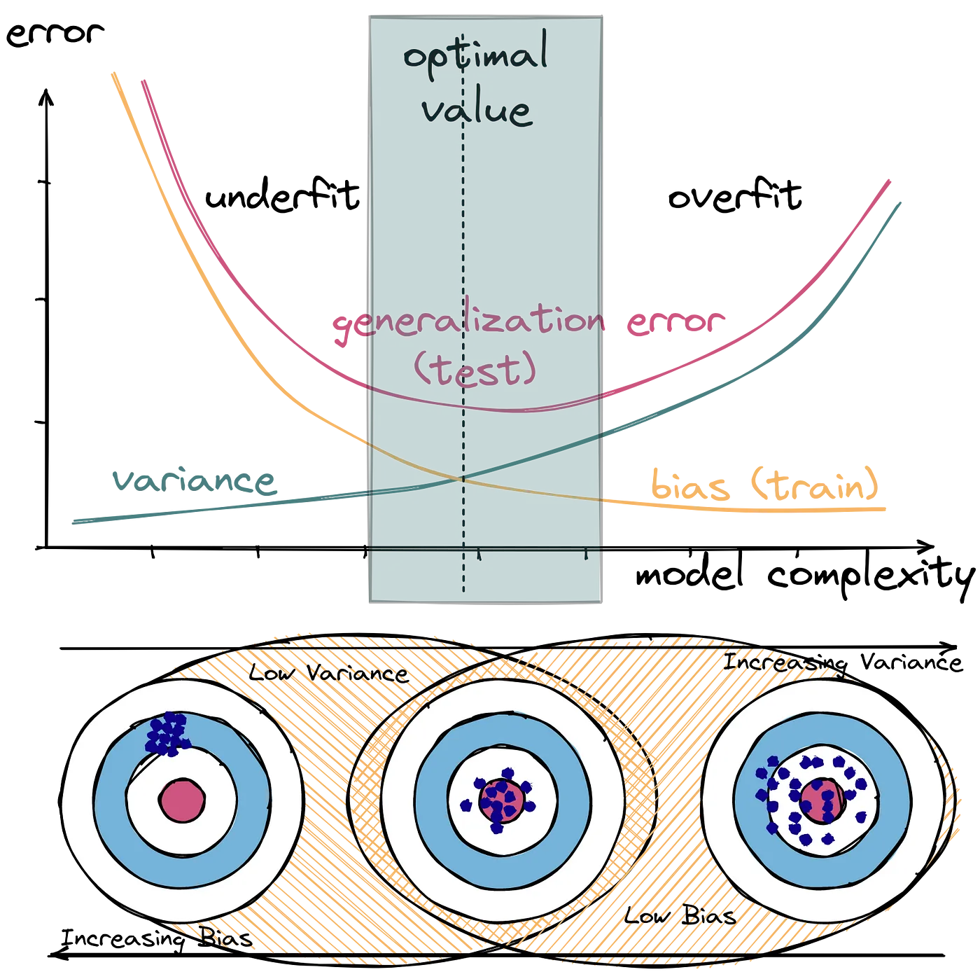
Overfitting
What is overfitting?
As the name subtly suggests, overfitting occurs when a model has learned too much. In particular, it has learned the training data so well, that beyond learning the underlying patterns in the data, it has also learned the noise in the data.
How do we know when overfitting has occurred?
- The model has a low train error, relative to training error for other models.
- The model has a high test error, relative to test error for other models.
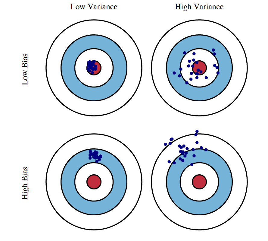
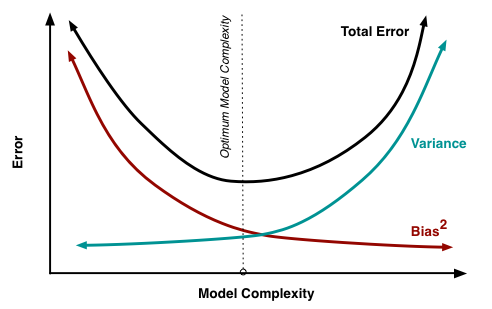
Bias-Variance Tradeoff
There are three sources of error in a model for supervised learning:
- Bias
- Variance
- Noise
The bias and variance make up the reducible error in a model. The noise is also called the irreducible error.
The bias of a model is the error due to the model’s assumptions or lack of flexibility. It is systematic error due to the model’s inability to (fully) learn the true underlying patterns in the data.
The variance of a model is the error due to the model’s sensitivity to the training data. It is the error due to the model (partially) learning some noise in the training data, and thus the model would change if the training data were changed.
Both bias and variance are related to the model’s flexibility.
- As flexibility increases, bias decreases.
- As flexibility increases, variance increases.
def simulate_sin_data(n, sd, seed):
np.random.seed(seed)
X = np.random.uniform(
low=-2 * np.pi,
high=2 * np.pi,
size=(n, 1),
)
signal = np.sin(X).ravel()
noise = np.random.normal(
loc=0,
scale=sd,
size=n,
)
y = signal + noise
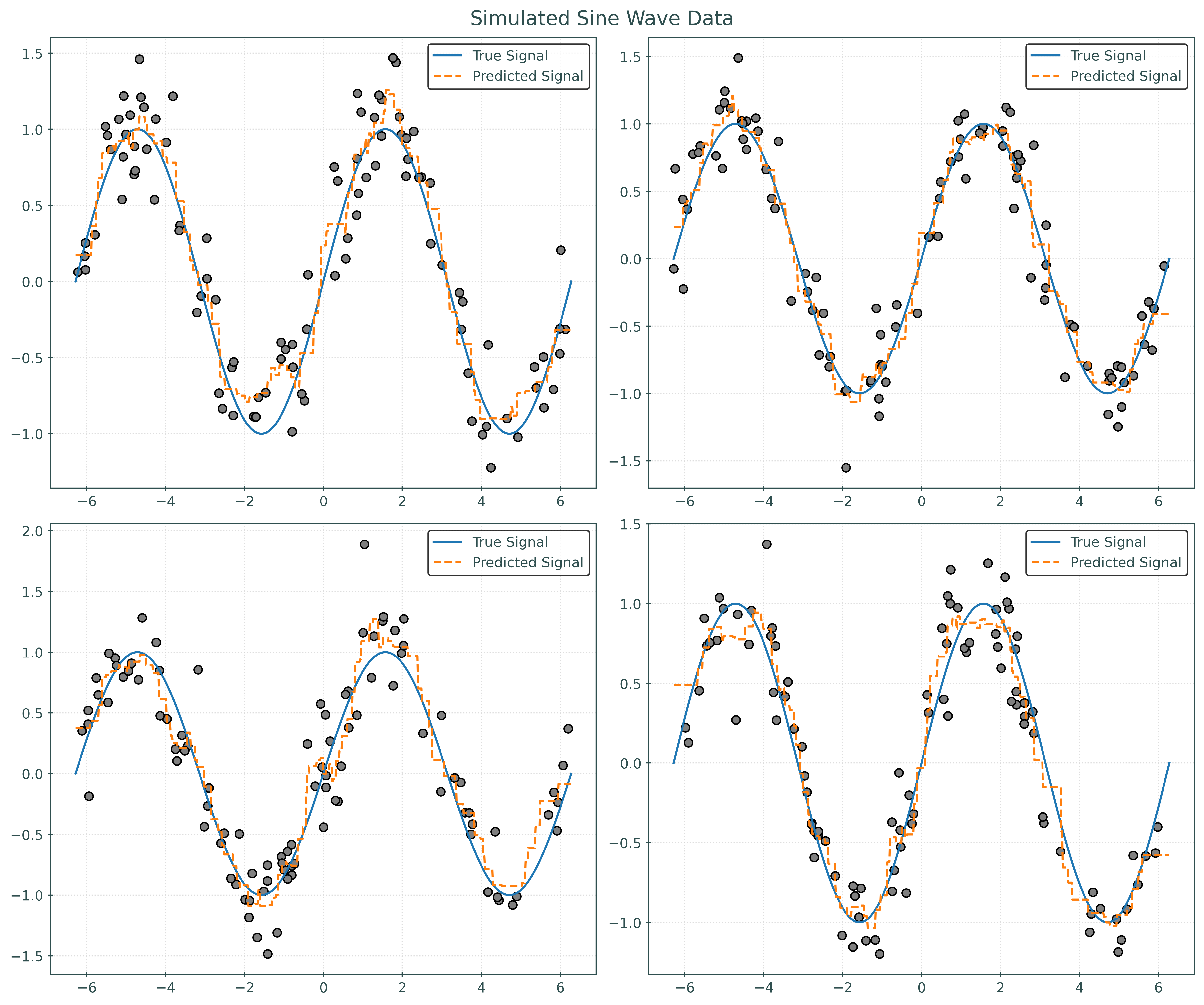
return X, ydef plot_four_simulations_and_predictions(n_neighbors):
fig, ax = plt.subplots(2, 2, figsize=(12, 10))
fig.suptitle("Simulated Sine Wave Data")
x_plot = np.linspace(-2 * np.pi, 2 * np.pi, 1000).reshape((-1, 1))
for i in range(2):
for j in range(2):
ax[i, j].plot(x_plot, np.sin(x_plot), label="True Signal")
X, y = simulate_sin_data(n=100, sd=0.25, seed=i * 2 + j)
ax[i, j].scatter(X, y, c="gray")
knn = KNeighborsRegressor(n_neighbors=n_neighbors)
knn.fit(X, y)
ax[i, j].plot(
x_plot,
knn.predict(x_plot),
label="Predicted Signal",
linestyle="--",
)
ax[i, j].legend()
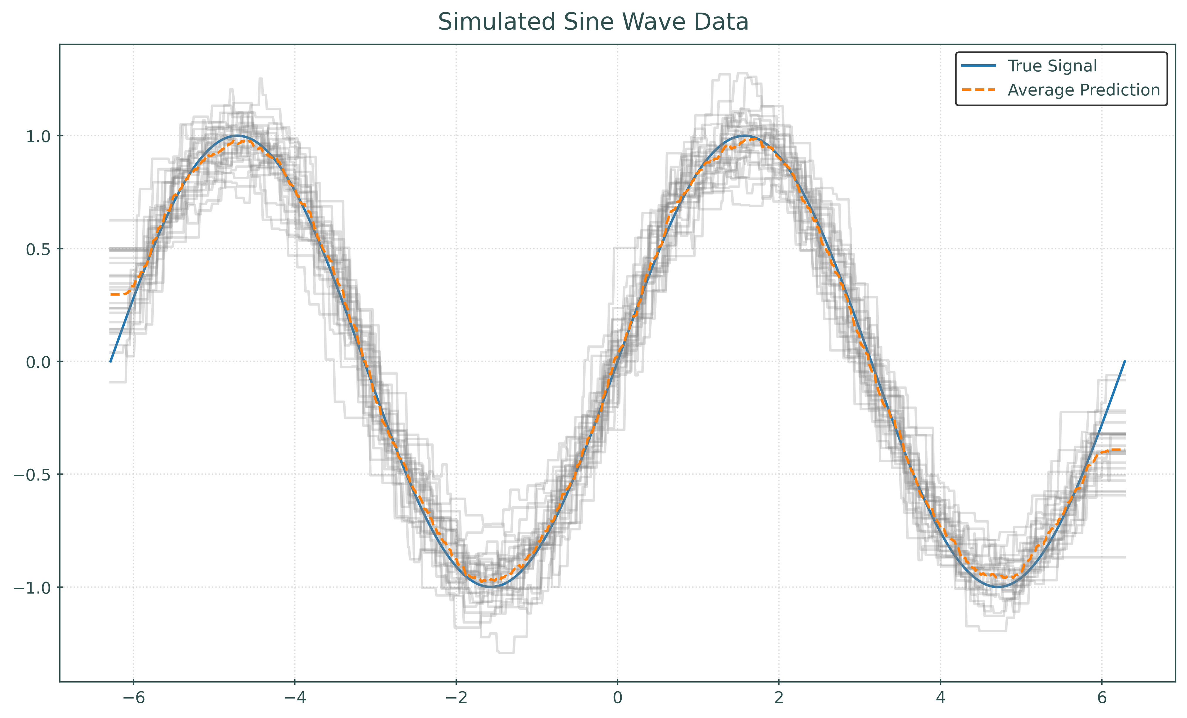
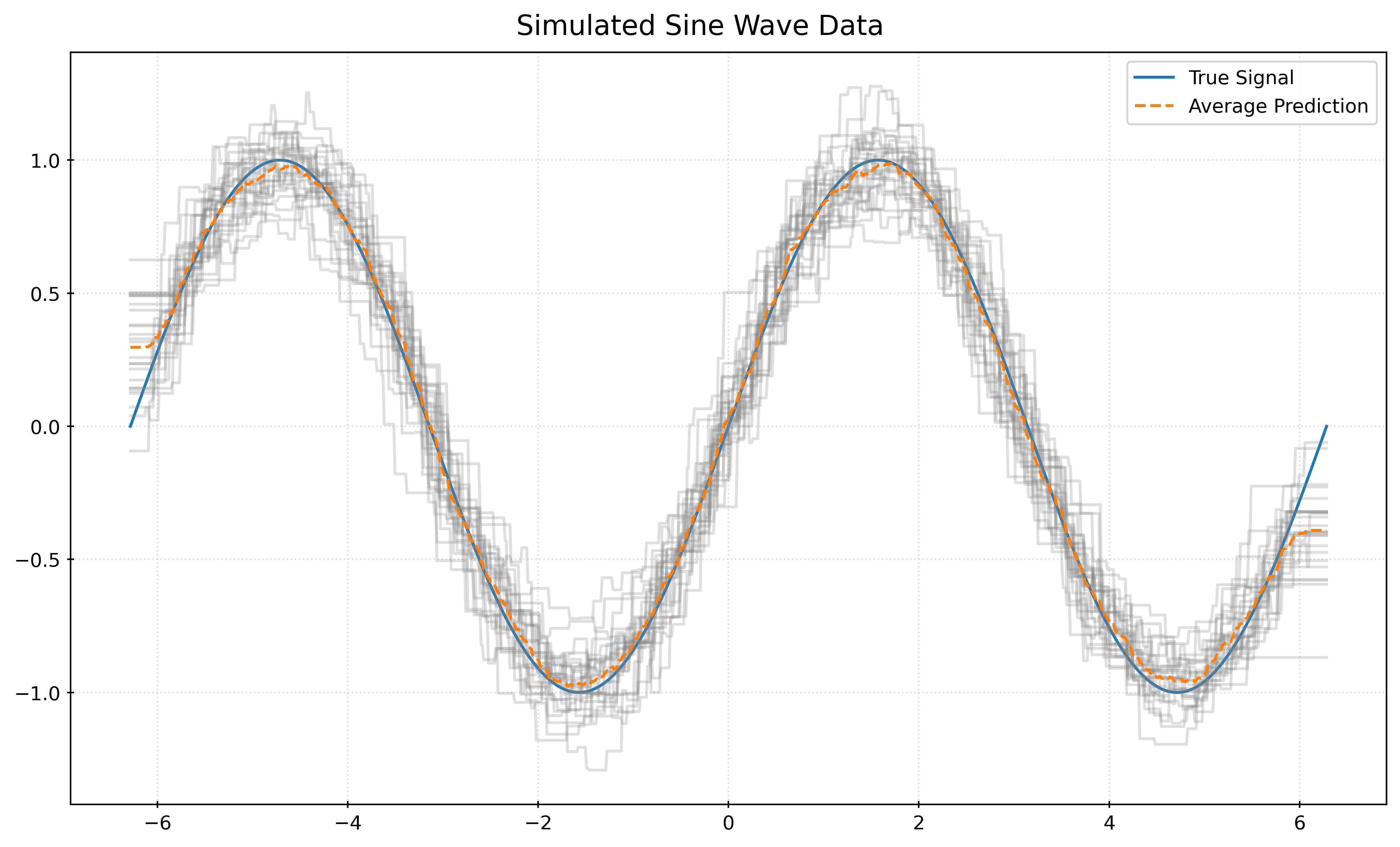
plt.show()def plot_many_simulations_and_predictions_with_average(n_neighbors):
fig, ax = plt.subplots(figsize=(10, 6))
fig.suptitle("Simulated Sine Wave Data")
x_plot = np.linspace(-2 * np.pi, 2 * np.pi, 1000).reshape((-1, 1))
ax.plot(x_plot, np.sin(x_plot), color="tab:blue", label="True Signal")
predictions = []
for seed in range(25):
X, y = simulate_sin_data(n=100, sd=0.25, seed=seed)
knn = KNeighborsRegressor(n_neighbors=n_neighbors)
knn.fit(X, y)
ax.plot(x_plot, knn.predict(x_plot), color="gray", alpha=0.25)
predictions.append(knn.predict(x_plot))
avg_prediction = np.mean(predictions, axis=0)
ax.plot(
x_plot,
avg_prediction,
color="tab:orange",
linestyle="--",
label="Average Prediction",
)
ax.legend()
plt.show()plot_four_simulations_and_predictions(100)
plot_many_simulations_and_predictions_with_average(100)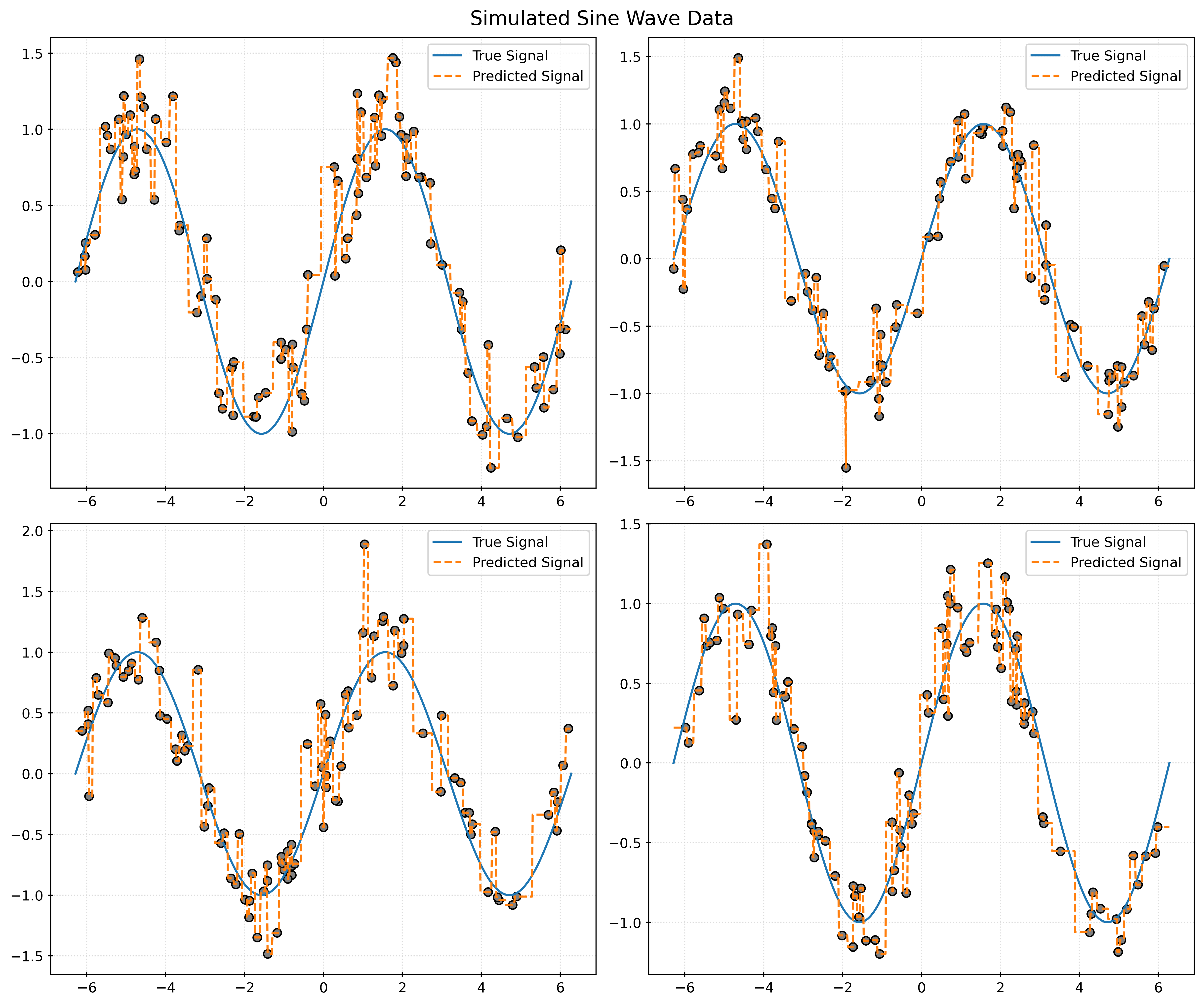

plot_four_simulations_and_predictions(1)
plot_many_simulations_and_predictions_with_average(1)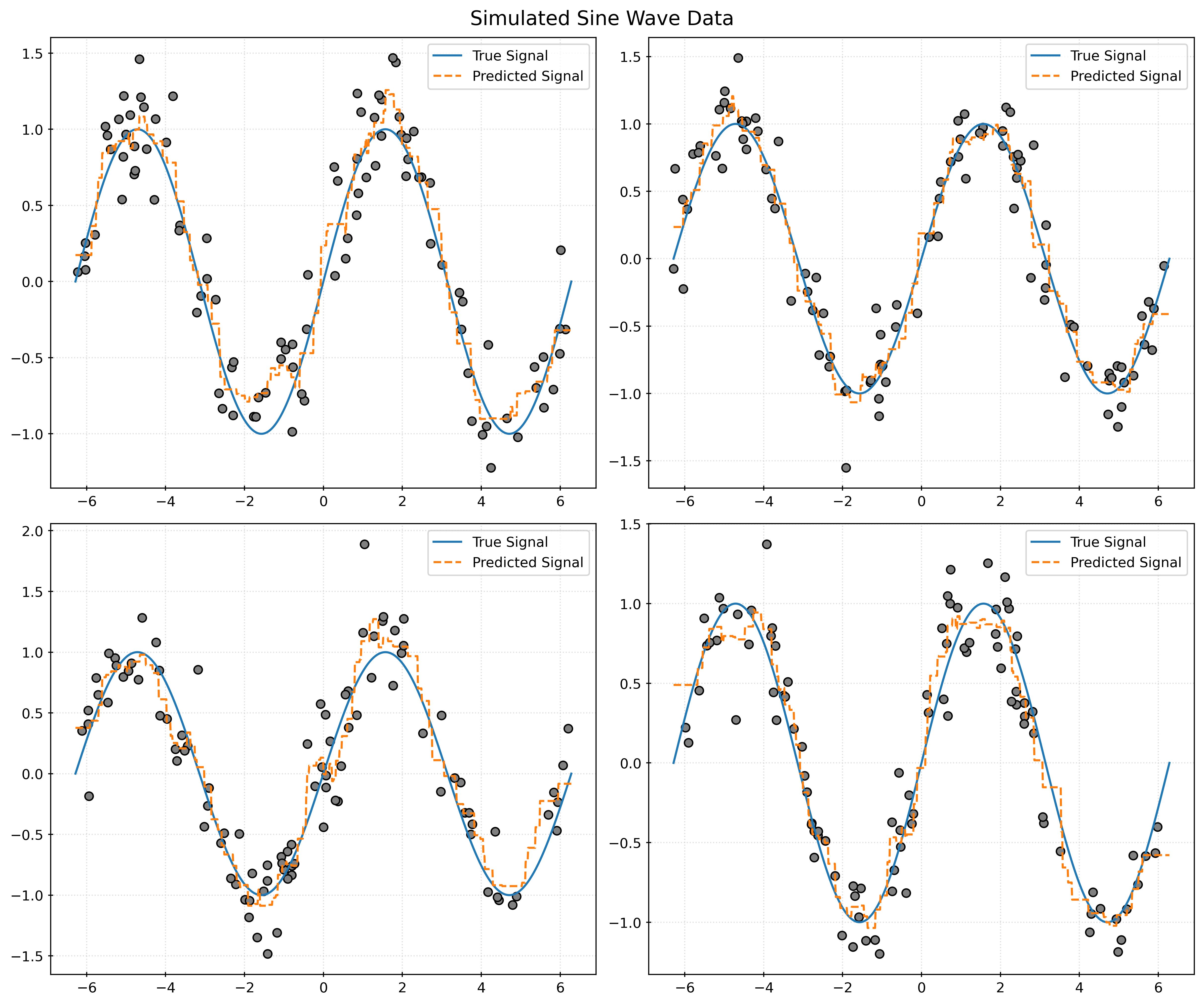
plot_four_simulations_and_predictions(5)
plot_many_simulations_and_predictions_with_average(5)