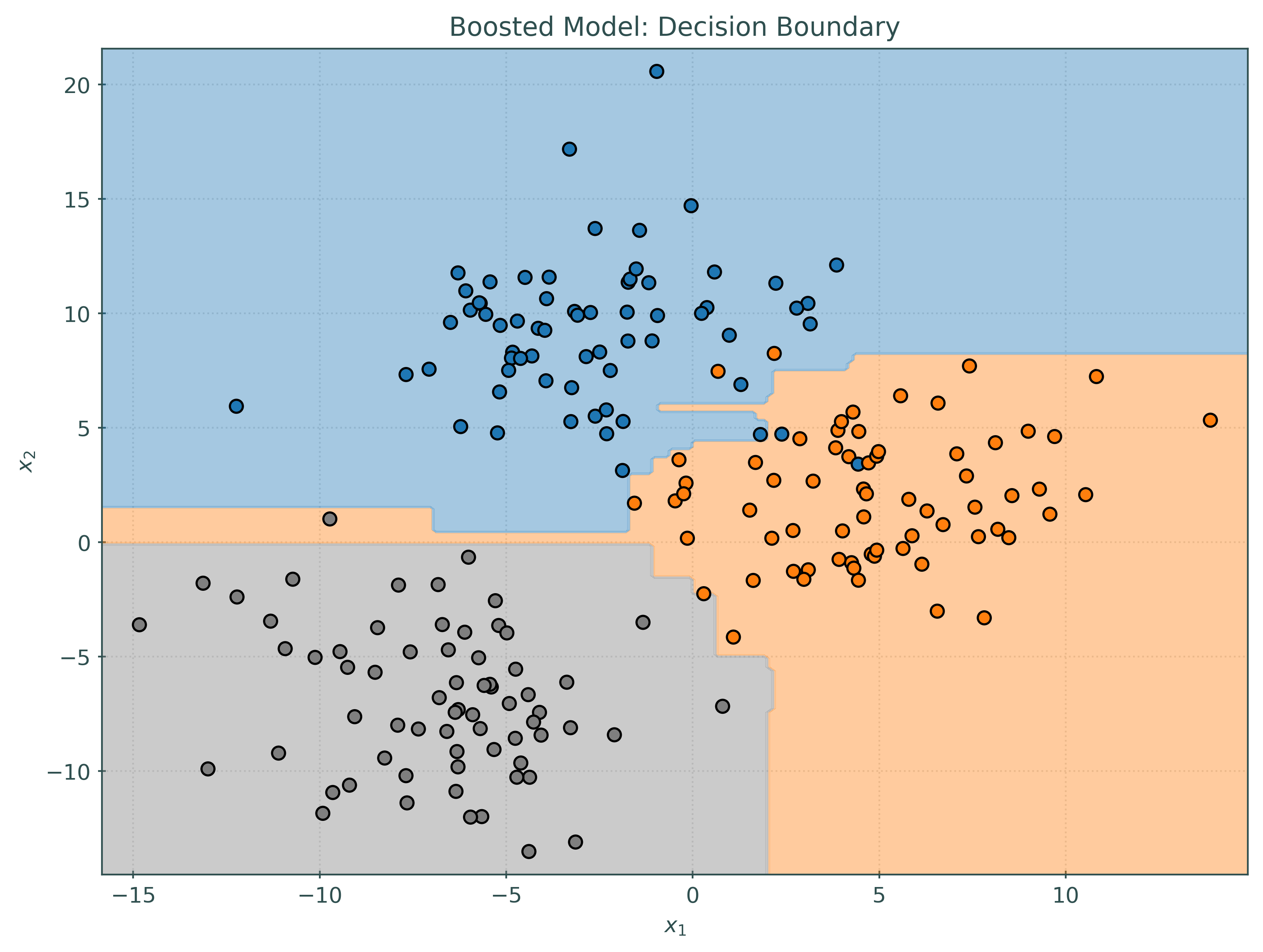
# general imports
import numpy as np
import pandas as pd
from joblib import parallel_backend

# data generation and loading
from sklearn.datasets import make_blobs
from sklearn.datasets import make_regression
from sklearn.datasets import load_breast_cancer
from sklearn.datasets import load_diabetes

# plotting
import matplotlib.pyplot as plt
import matplotlib.colors
from sklearn.inspection import DecisionBoundaryDisplay
from sklearn.tree import plot_tree
from sklearn.tree import export_text

# basic classification
from sklearn.tree import DecisionTreeClassifier
from sklearn.neighbors import KNeighborsClassifier
from sklearn.linear_model import LogisticRegression

# basic regression
from sklearn.tree import DecisionTreeRegressor
from sklearn.neighbors import KNeighborsRegressor
from sklearn.linear_model import LinearRegression

# ensembles for classification
from sklearn.ensemble import VotingClassifier
from sklearn.ensemble import RandomForestClassifier
from sklearn.ensemble import HistGradientBoostingClassifier

# ensembles for regression
from sklearn.ensemble import VotingRegressor
from sklearn.ensemble import RandomForestRegressor
from sklearn.ensemble import HistGradientBoostingRegressor

# model tuning and preprocessing
from sklearn.model_selection import train_test_split
from sklearn.model_selection import GridSearchCV
from sklearn.pipeline import Pipeline

# model metrics
from sklearn.metrics import root_mean_squared_error
from sklearn.metrics import accuracy_scoreEnsembles
Using the Wisdom of Crowds
Setup
In this note, we will investigate the use of ensemble methods for supervised learning.
# helper function to plot decision boundaries
def plot_decision_boundary(model, X, y, model_name):
    cmap = matplotlib.colors.ListedColormap(
        ["tab:blue", "tab:orange", "tab:gray"],
    )
    _, ax = plt.subplots(figsize=(8, 6))
    DecisionBoundaryDisplay.from_estimator(
        model,
        X,
        response_method="predict",
        grid_resolution=200,
        alpha=0.4,
        xlabel="$x_1$",
        ylabel="$x_2$",
        ax=ax,
        cmap=cmap,
    )
    ax.scatter(
        X[:, 0],
        X[:, 1],
        c=y,
        edgecolor="k",
        cmap=cmap,
    )
    ax.set_title(f"{model_name}: Decision Boundary")
    plt.show()
# helper function to simulate some example data
def generate_example_data(n=10, seed=None):
np.random.seed(seed)
data = {
"Age": np.random.randint(
18,
70,
size=n,
),
"Income": np.random.randint(
50000,
150000,
size=n,
),
"Education": np.random.choice(
["High School", "Bachelor", "Master", "PhD"],
size=n,
),
}
df = pd.DataFrame(data)
return df# function to simulate data (in numpy) for regression task
def simulate_sin_data(n=25, seed=42):
np.random.seed(seed)
X = np.random.uniform(low=-2 * np.pi, high=2 * np.pi, size=(n, 1))
e = np.random.normal(loc=0, scale=0.25, size=(n, 1))
y = np.sin(X) + e
y = y.ravel()
return X, y
# helper function for plotting sin data and learned regression model
def plot_sin_regression(model, X_train, y_train, title, ax=None):
x_plot = np.linspace(-2 * np.pi, 2 * np.pi, 1000)
x_plot = x_plot.reshape((1000, 1))
if ax is None:
fig, ax = plt.subplots()
ax.scatter(
X_train,
y_train,
label="Actual",
zorder=3,
c="tab:blue",
alpha=0.75,
)
ax.plot(
x_plot,
model.predict(x_plot),
color="tab:gray",
label="Fitted",
)
ax.set_xlabel("$x$")
ax.set_ylabel("$y$")
ax.set_ylim(-3, 3)
ax.legend()
ax.set_title(title)# helper function to better display results of cross-validation
def cv_results_to_df(cv_results):
params = pd.DataFrame(cv_results["params"])
params.columns = [col.split("__")[-1] for col in params.columns]
scores = pd.DataFrame(
{
"mean_test_score": cv_results["mean_test_score"],
"std_test_score": cv_results["std_test_score"],
}
)
results_df = pd.concat([params, scores], axis=1)
results_df["mean_test_score"] = results_df["mean_test_score"].map("{:.2f}".format)
results_df["std_test_score"] = results_df["std_test_score"].map("{:.2f}".format)
return results_dfSome Review
Let \(X_1, X_2, \dots, X_n \sim F\), where each \(X_i\) has:
- population mean \(\mu = \mathbb{E}[X_i]\),
- population variance \(\sigma^2 = \text{Var}(X_i)\).
Recall that the sample mean is defined as:
\[ \bar{X} = \frac{1}{n} \sum_{i=1}^{n} X_i \]
The expected value (mean) of the sample mean is:
\[ \mathbb{E}[\bar{X}] = \mu. \]
If we can additionally assume that the \(X_i\) are independent, the variance of the sample mean is:
\[ \text{Var}(\bar{X}) = \frac{\sigma^2}{n}. \]
Importantly: The variance of an average is smaller (proportional to the sample size) than the variance of an individual observation.
However, if we cannot make the independence assumption, the variance has an additional term:
\[ \text{Var}(\bar{X}) = \frac{\sigma^2}{n} + \text{(an additional term that depends on the covariances)}. \]
For our purposes, the specifics of this terms is not important, only that it exists, and the stronger the covariance, the larger the term. To the extent that we have control, we will seek to reduce the covariances to keep variances low.
Key Ideas
Ensembles are conceptually very simple. An ensemble is simply a model that is a combination of other models. Often, ensembles are created through the following general process:
- Fit “many” models to train data.
- These models are called the base learners.
- “Many” can be as few as two or as many as a computer’s memory will allow.
- Make predictions with each model that was fit.
- “Average” these predictions to make a prediction from the ensemble.
- For regression: literally average the predictions.
- For classification: different “voting” mechanisms available.
- “Average” these predictions to make a prediction from the ensemble.
We will consider “custom” ensembles using VotingRegressor() and VotingClassifier(), but more importantly we will look at two general forms of ensembles:
- Bagging (“Bootstrap Aggregation”)
- Boosting
How and why do these methods work?
- Bagging uses many strong base learners in parallel and attempts to reduce the variance of the base learners through averaging.
- A strong learner is very effective at learning the training data and thus is likely to overfit.
- Boosting uses many weak base learners in sequence and attempts to reduce the bias of the base learners.
- A weak learner is potentially unable to learn the training data well and thus is likely to underfit.
For bagging, we will focus on a particular variant called a random forest, which as the name suggests, uses a collection of decision trees.
For boosting, we will focus on a modern algorithm called histogram gradient boosting which is inspired by the popular and effective LightGBM.
Each of these methods can be used for both regression and classification.
Custom (Voting) Regression Ensemble
Using VotingRegressor(), we can easily create a custom ensemble for regression.
# simulate some data for regression
X, y = make_regression(
    n_samples=300,
    n_features=5,
    noise=0.3,
    random_state=42,
)

# train-test split the data
X_train, X_test, y_train, y_test = train_test_split(
    X,
    y,
    test_size=0.25,
    random_state=42,
)
# create three (different) base learners
linear = LinearRegression()
knn = KNeighborsRegressor()
tree = DecisionTreeRegressor(random_state=42)# fit the base learners
_ = linear.fit(X_train, y_train)
_ = knn.fit(X_train, y_train)
_ = tree.fit(X_train, y_train)# make predictions on (some) of the test observations
predictions = (
linear.predict(X_test[:3]),
tree.predict(X_test[:3]),
knn.predict(X_test[:3]),
)
predictions(array([-32.15932366, -22.28278917, 2.22604893]),
array([-10.61666369, -26.73985752, 47.73921455]),
array([-18.96972927, -15.03687023, 7.67073112]))# create a custom ensemble using the base learners
ensemble = VotingRegressor(
[
("linear", linear),
("knn", knn),
("tree", tree),
]
)
ensembleVotingRegressor(estimators=[('linear', LinearRegression()),
('knn', KNeighborsRegressor()),
('tree', DecisionTreeRegressor(random_state=42))])In a Jupyter environment, please rerun this cell to show the HTML representation or trust the notebook. On GitHub, the HTML representation is unable to render, please try loading this page with nbviewer.org.
VotingRegressor(estimators=[('linear', LinearRegression()),
                            ('knn', KNeighborsRegressor()),
('tree', DecisionTreeRegressor(random_state=42))])LinearRegression()
KNeighborsRegressor()
DecisionTreeRegressor(random_state=42)
# fit the custom ensemble
_ = ensemble.fit(X_train, y_train)
# make predictions on (some) of the test observations
ensemble.predict(X_test[:3])array([-20.58190554, -21.35317231, 19.2119982 ])# average the predictions from the base learners
np.mean(predictions, axis=0)array([-20.58190554, -21.35317231, 19.2119982 ])Notice that we have verified that the predictions from the ensemble are indeed the average of the predictions from the base learners.
Custom (Voting) Classification Ensemble
Using VotingClassifier(), we can easily create custom ensembles for classification.
# simulate some data for classification
X, y = make_blobs(
    n_samples=400,
    cluster_std=3,
    random_state=42,
)

# train-test split the data
X_train, X_test, y_train, y_test = train_test_split(
    X,
    y,
    test_size=0.50,
    random_state=42,
)
# create three (different) base learners
logistic = LogisticRegression()
knn = KNeighborsClassifier()
tree = DecisionTreeClassifier(random_state=42)# fit the base learners
_ = logistic.fit(X_train, y_train)
_ = knn.fit(X_train, y_train)
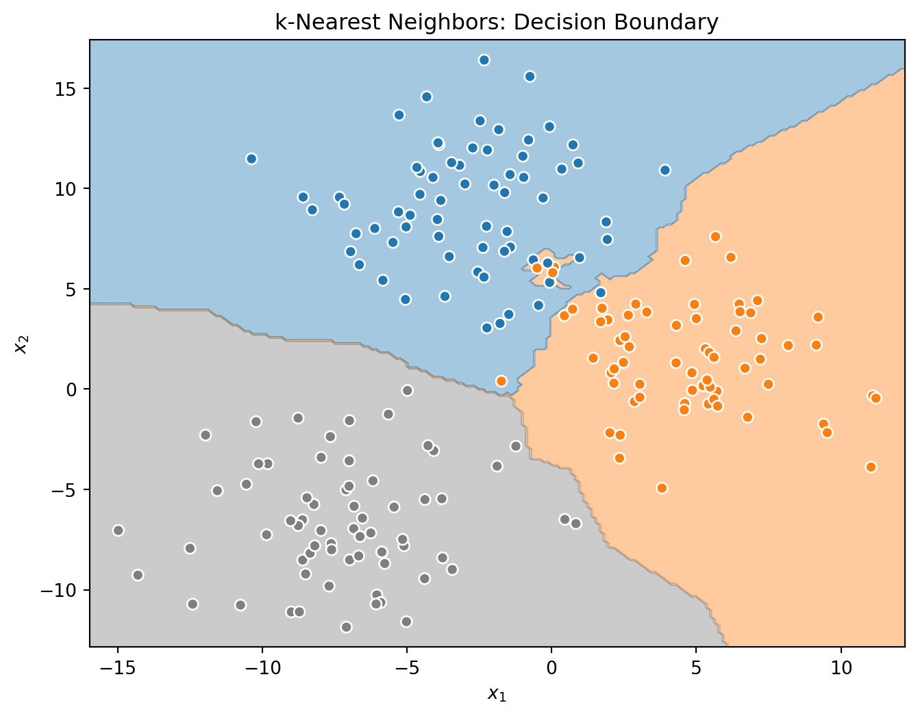
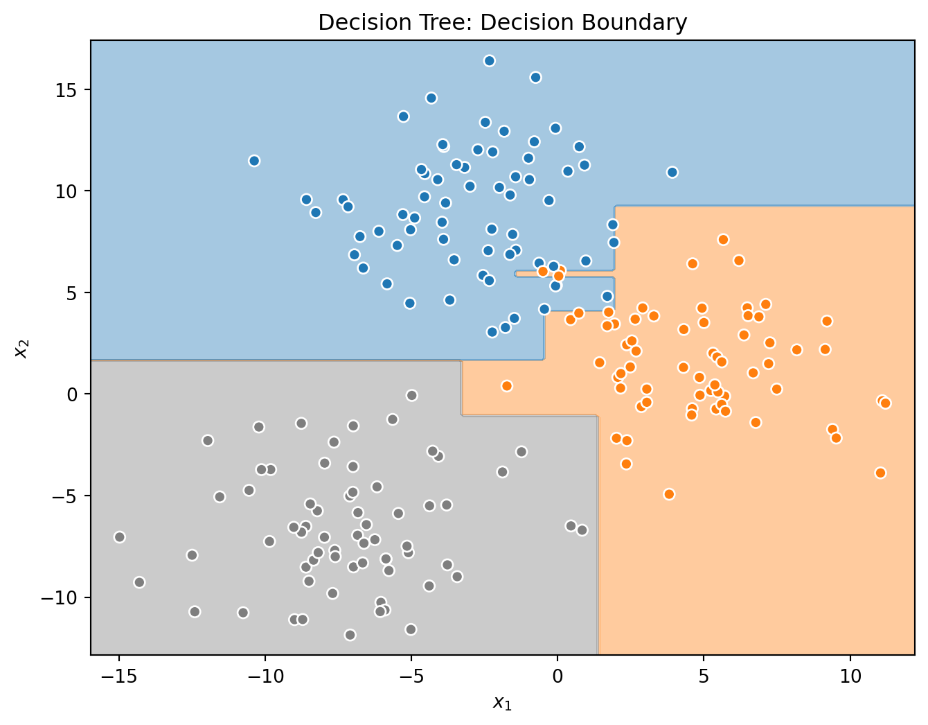
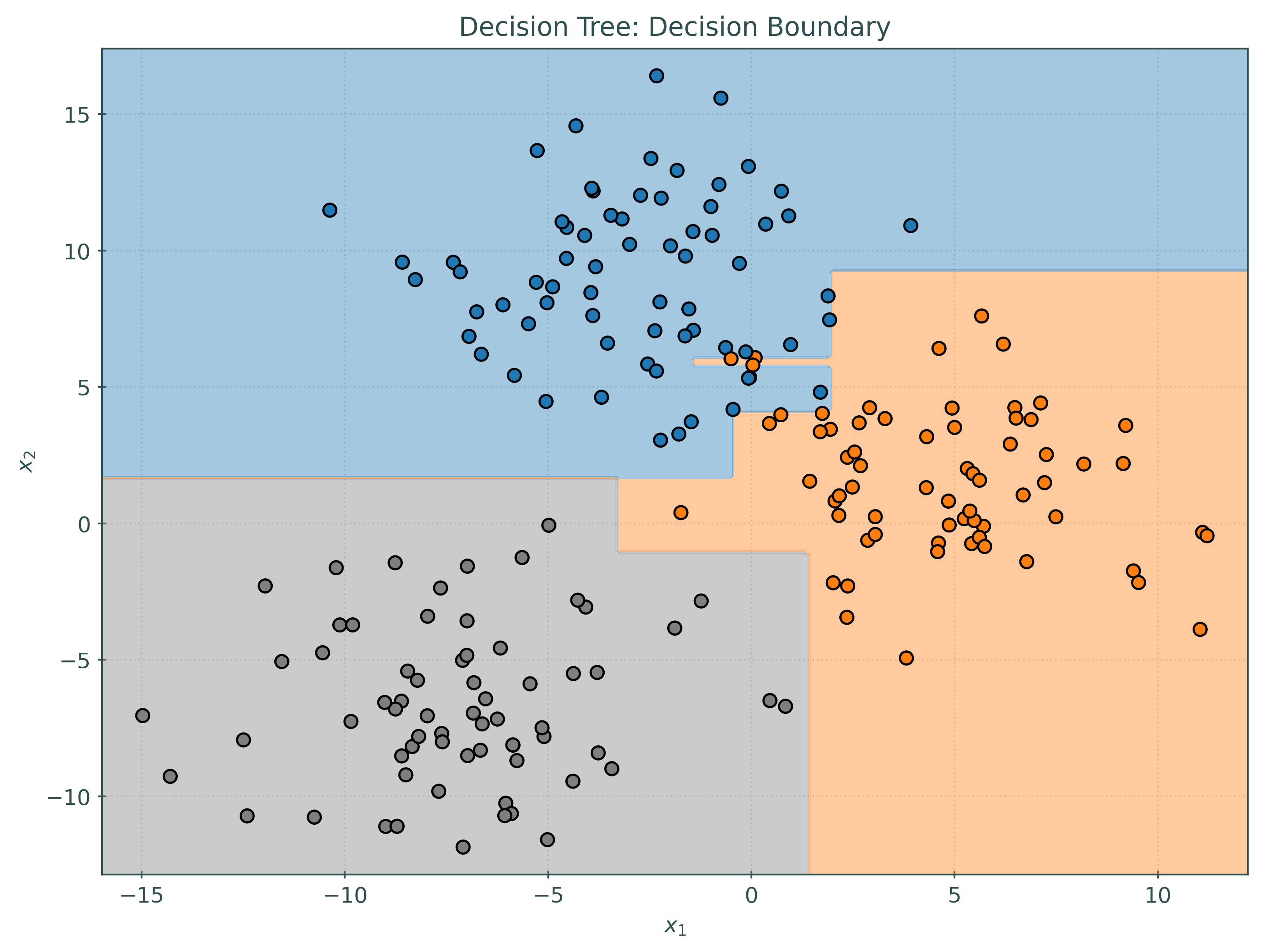
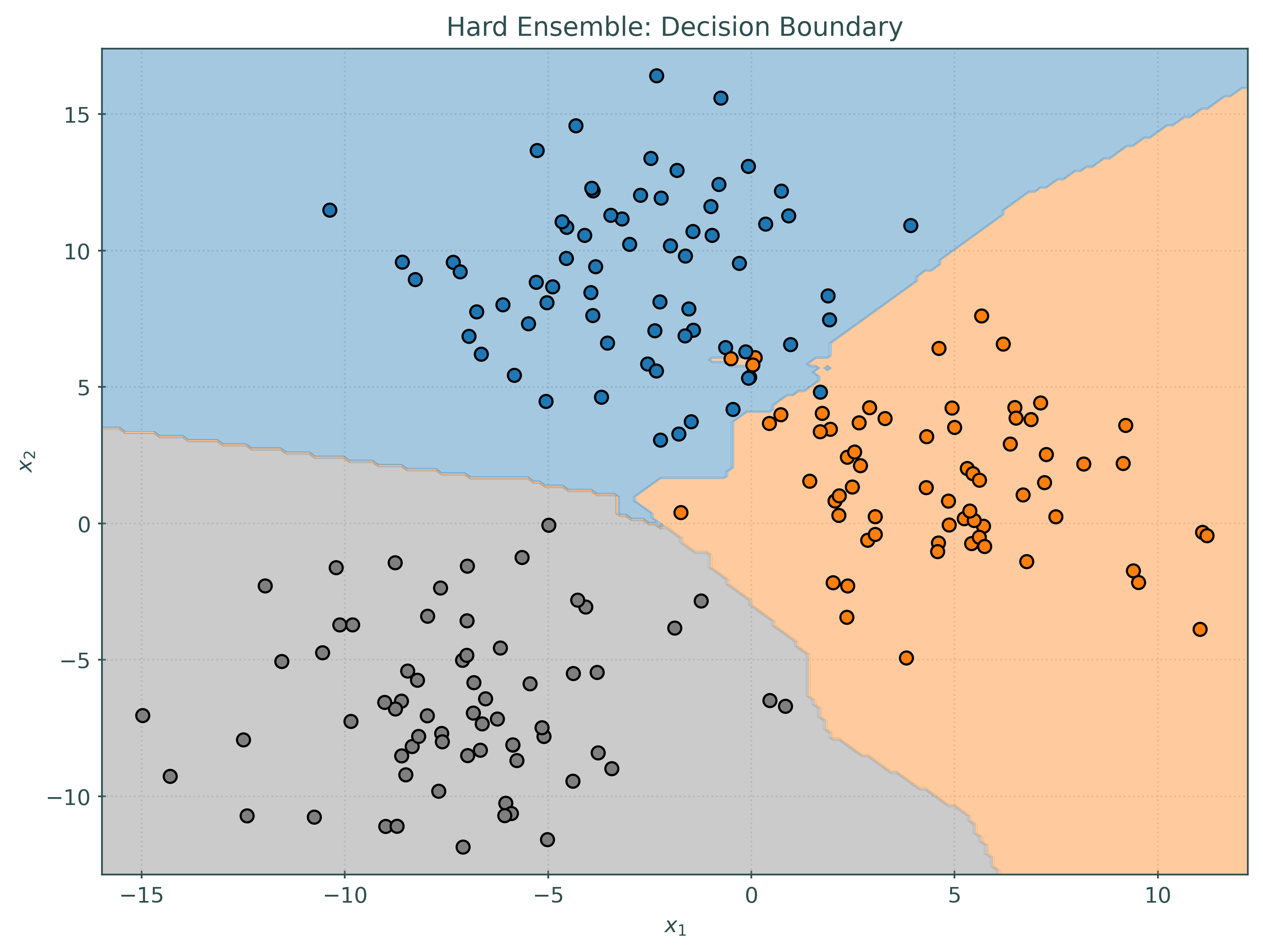
_ = tree.fit(X_train, y_train)Before investigating the voting classifier, let’s first look at the decision boundaries created by the three base learners.
# create a custom soft voting ensemble using the base learners
ensemble_soft = VotingClassifier(
    [
        ("logistic", logistic),
        ("knn", knn),
        ("tree", tree),
    ],
    voting="soft",
)
ensemble_soft
VotingClassifier(estimators=[('logistic', LogisticRegression()),
('knn', KNeighborsClassifier()),
('tree', DecisionTreeClassifier(random_state=42))],
voting='soft')In a Jupyter environment, please rerun this cell to show the HTML representation or trust the notebook. On GitHub, the HTML representation is unable to render, please try loading this page with nbviewer.org.
VotingClassifier(estimators=[('logistic', LogisticRegression()),
                             ('knn', KNeighborsClassifier()),
                             ('tree', DecisionTreeClassifier(random_state=42))],
voting='soft')LogisticRegression()
KNeighborsClassifier()
DecisionTreeClassifier(random_state=42)
# fit the custom ensemble
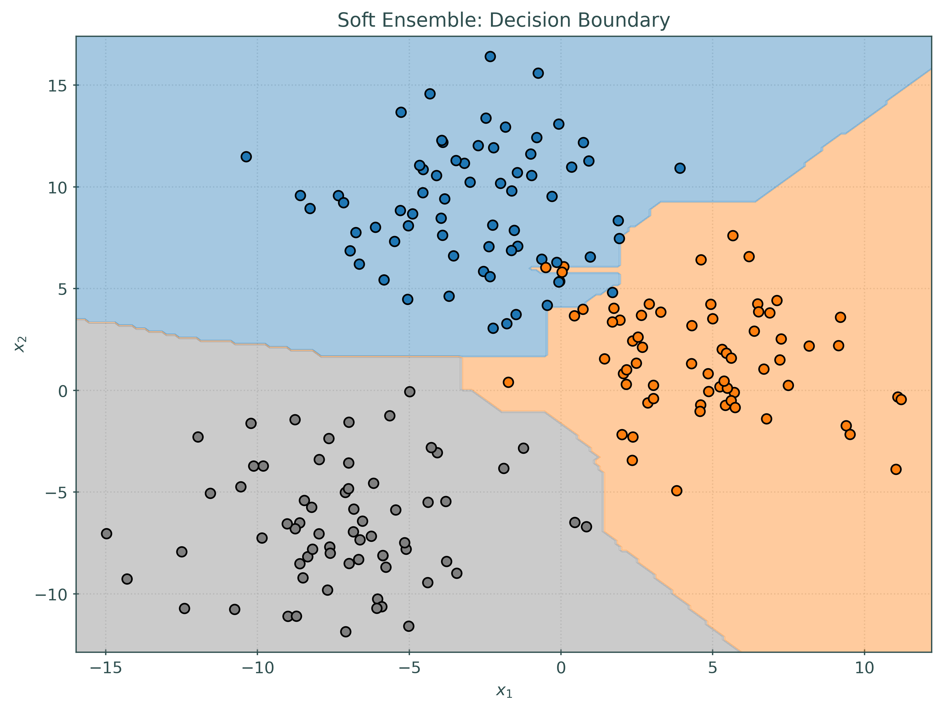
_ = ensemble_soft.fit(X_train, y_train)Notice that the decision boundary for the soft voting classifier is quite different than each of the base learners, but in some sense contains patterns from each of the base learners.
# create a custom hard voting ensemble using the base learners
ensemble_hard = VotingClassifier(
    [
        ("logistic", logistic),
        ("knn", knn),
        ("tree", tree),
    ],
    voting="hard",
)
ensemble_hard
VotingClassifier(estimators=[('logistic', LogisticRegression()),
('knn', KNeighborsClassifier()),
('tree', DecisionTreeClassifier(random_state=42))])In a Jupyter environment, please rerun this cell to show the HTML representation or trust the notebook. On GitHub, the HTML representation is unable to render, please try loading this page with nbviewer.org.
VotingClassifier(estimators=[('logistic', LogisticRegression()),
                             ('knn', KNeighborsClassifier()),
('tree', DecisionTreeClassifier(random_state=42))])LogisticRegression()
KNeighborsClassifier()
DecisionTreeClassifier(random_state=42)
# fit the custom ensemble
_ = ensemble_hard.fit(X_train, y_train)What is the difference between soft voting and hard voting?
- Hard Voting: Predict the class with the most votes from the base models.
- Soft Voting. Predict the class with the largest average probability from the base learners.
For example consider five learners for a classification task. The target value has possible values A, B, and C. For each learner, we have a prediction and estimated probabilities (of [A, B, C]) for a single observation.
- Learner 1
- Prediction:
A - Probabilities;
[0.6, 0.0, 0.4]
- Prediction:
- Learner 2
- Prediction:
B - Probabilities:
[0.3, 0.4, 0.3]
- Prediction:
- Learner 3
- Prediction:
C - Probabilities:
[0.1, 0.0, 0.9]
- Prediction:
- Learner 4
- Prediction:
B - Probabilities:
[0.2, 0.5, 0.3]
- Prediction:
- Learner 5
- Prediction:
B - Probabilities:
[0.2, 0.5, 0.3]
- Prediction:
Using hard voting, we see there are three learners predicting B, thus this is the majority vote, and the prediction made via hard voting.
With soft voting, we must first average the probabilities, which gives: [0.28, 0.28, 0.44]. Thus, because the C class has the highest probability, the prediction made with soft voting is C.
# make predictions on (some) of the test observations
some_test_predictions = X_test[20:30]
predictions = (
    logistic.predict(some_test_predictions),
    knn.predict(some_test_predictions),
    tree.predict(some_test_predictions),
)
predictions
(array([1, 1, 2, 1, 2, 1, 2, 0, 1, 2]),
array([1, 1, 2, 1, 2, 1, 2, 0, 1, 2]),
array([1, 1, 2, 1, 2, 2, 2, 0, 1, 2]))# make predictions on (some) of the test observations
ensemble_hard.predict(some_test_predictions)array([1, 1, 2, 1, 2, 1, 2, 0, 1, 2])# make predictions on (some) of the test observations
ensemble_soft.predict(some_test_predictions)array([1, 1, 2, 1, 2, 2, 2, 0, 1, 2])While most of the predictions are the same, notice that the hard and soft voting classifiers make slightly different predictions, in this case, on one particular observation. You can see this effect more generally by comparing the plots of the decision boundaries above.
# get probabilities for a test observation
single_test_obs = X_test[[20]]
probabilities = (
    logistic.predict_proba(single_test_obs),
    knn.predict_proba(single_test_obs),
    tree.predict_proba(single_test_obs),
)
probabilities
(array([[0.14546585, 0.8438736 , 0.01066055]]),
array([[0.4, 0.6, 0. ]]),
array([[0., 1., 0.]]))Note that it is not possible to obtain probabilities with a hard voting ensemble in sklearn. Attempting to do so would produce the following error:
AttributeError: predict_proba is not available when voting='hard'
# get probabilities for a test observation
ensemble_soft.predict_proba(single_test_obs)
array([[0.18182195, 0.81462453, 0.00355352]])# average probabilities from the base learners
np.mean(probabilities, axis=0)array([[0.18182195, 0.81462453, 0.00355352]])Notice that the average of the probabilities from the base learners is the same as the probabilities obtained from the soft voting classifier.
The Bootstrap
Before introducing random forests, we take a quick detour to describe the bootstrap.
Bootstrapping is a powerful and important technique in statistics developed by Bradley Efron in the late 1970s and early 1980s.
While the bootstrap has many uses, we will narrowly focus on the resampling aspect of the method. That is, generating datasets that are similar (appear to have been sampled from the same distribution as the original dataset) but contain different observations.
example_sample = generate_example_data(seed=42)
example_sample| Age | Income | Education | |
|---|---|---|---|
| 0 | 56 | 87194 | PhD |
| 1 | 69 | 137498 | Bachelor |
| 2 | 46 | 94131 | Bachelor |
| 3 | 32 | 110263 | Bachelor |
| 4 | 60 | 66023 | PhD |
| 5 | 25 | 91090 | PhD |
| 6 | 38 | 117221 | High School |
| 7 | 56 | 114820 | High School |
| 8 | 36 | 50769 | PhD |
| 9 | 40 | 109735 | Bachelor |
A bootstrap resample is a dataset that has the same dimension as the original data, importantly the same number of observations. These observations are sampled with replacement.
# function to produce a bootstrap resample
def generate_bootstrap_resample(df, seed=None):
    resample = df.sample(
        n=len(df),
        replace=True,
        random_state=seed,
    )
    return resample
We’ll generate three new bootstrap resamples based on the example_sample data. Importantly, you should notice two things about each bootstrap resample:
- Sometimes, an original observation is duplicated,
- Sometimes, an original observation is not included.
Pay attention to the printed index which will make these easy to see.
generate_bootstrap_resample(example_sample, seed=1)| Age | Income | Education | |
|---|---|---|---|
| 5 | 25 | 91090 | PhD |
| 8 | 36 | 50769 | PhD |
| 9 | 40 | 109735 | Bachelor |
| 5 | 25 | 91090 | PhD |
| 0 | 56 | 87194 | PhD |
| 0 | 56 | 87194 | PhD |
| 1 | 69 | 137498 | Bachelor |
| 7 | 56 | 114820 | High School |
| 6 | 38 | 117221 | High School |
| 9 | 40 | 109735 | Bachelor |
generate_bootstrap_resample(example_sample, seed=2)| Age | Income | Education | |
|---|---|---|---|
| 8 | 36 | 50769 | PhD |
| 8 | 36 | 50769 | PhD |
| 6 | 38 | 117221 | High School |
| 2 | 46 | 94131 | Bachelor |
| 8 | 36 | 50769 | PhD |
| 7 | 56 | 114820 | High School |
| 2 | 46 | 94131 | Bachelor |
| 1 | 69 | 137498 | Bachelor |
| 5 | 25 | 91090 | PhD |
| 4 | 60 | 66023 | PhD |
generate_bootstrap_resample(example_sample, seed=3)| Age | Income | Education | |
|---|---|---|---|
| 8 | 36 | 50769 | PhD |
| 9 | 40 | 109735 | Bachelor |
| 3 | 32 | 110263 | Bachelor |
| 8 | 36 | 50769 | PhD |
| 8 | 36 | 50769 | PhD |
| 0 | 56 | 87194 | PhD |
| 5 | 25 | 91090 | PhD |
| 3 | 32 | 110263 | Bachelor |
| 9 | 40 | 109735 | Bachelor |
| 9 | 40 | 109735 | Bachelor |
The “trick” employed by the bootstrap is that each bootstrap resample could be considered a “new” random sample from the population. Of course this is not actually the case, and thus there are limitations to the bootstrap, however it often works well when the original random sample is quite large. We’ll skip these details for now. We are simply interested in being able to generate these bootstrap resamples.
Random Forest
As you might imagine from the name, a random forest is a collection of trees. The “random” in random forests is usually introduced through two distinct sources.
Suppose we fit 100 decision trees, each to the same training data. This would be an odd thing to do, because each of these trees will make the same predictions! Averaging them would be no different than using a single tree. The predictions from these trees would be perfectly correlated! And thus, we’d see exactly zero reduction in variance from using this procedure.
How can we de-correlate (reduce covariance) between the base learners? Add randomness to decrease correlation between the base learners. This might seem quite odd because in some sense, we are adding variability to each individual tree. But it turns out that doing so will reduce the variance of an ensemble that leverages these base learners with added randomness.
With sufficiently de-correlated trees, averaging the predictions from the trees significantly reduces variance compared to a single tree.
How do we add this randomness to individual trees?
- Use “different” data when fitting each tree.
- Add randomness when determining the splits for each tree.
To address the first, we will use bootstrap resamples. Fitting trees to bootstrap resamples will “de-correlate” the trees in that they will not always produce the same predictions.
To address the second, we will modify the usual tree fitting procedure. Recall the parameters available when fitting a decision tree.
DecisionTreeRegressor().get_params(){'ccp_alpha': 0.0,
'criterion': 'squared_error',
'max_depth': None,
'max_features': None,
'max_leaf_nodes': None,
'min_impurity_decrease': 0.0,
'min_samples_leaf': 1,
'min_samples_split': 2,
'min_weight_fraction_leaf': 0.0,
'monotonic_cst': None,
'random_state': None,
'splitter': 'best'}You may have wondered: Why is there a random_state parameter? What randomness would we ever need to control for reproducibility?
The max_features parameter is the answer to this question. By default, with a value of None, decision trees consider all feature variables when determining the best split of each node during the fitting process. However, this parameter allows us to alter this part of the process. We can limit the number of features considered for each split, at random. That is, if we set max_features=1, the most extreme case, when determining a split, rather than consider all available features, we first randomly select a feature, then find the best possible split of the available splits with only that feature.
Note that, this randomly selected feature is not used for all splits. Instead, each time the method attempts a split, it randomly chooses a feature.
This parameter can be set to be any value between 1 and the number of features available. Using 1 adds the most variability to the fitting procedure, and thus de-correlates the trees as much as possible. Using all features does not add any variability, and thus provides no additional de-correlation. (De-correlation would still be introduced via the bootstrap resampling.) Eventually, we will consider this parameter a tuning parameter of random forests. Setting another integer value for this parameter, say 2, would consider splits of 2 randomly chosen features.
As seen in the documentation, there are two built-in options for max_features that can be expressed as strings:
- If
"sqrt", thenmax_features=sqrt(n_features). - If
"log2", thenmax_features=log2(n_features).
These two options are well supported in the literature, and we will see that "sqrt" is recommended for random forests. While we can tune this parameter, it is generally not worthwhile. It often provides little benefit, but incurs a large computational cost.
The trees fit and then combined to produce a random forest are generally strong learners. Specifically for decision trees, that generally means that each individual tree will likely be overfit, specifically by growing a very deep tree. Trees in random forests are often unconstrained in any way, splitting until each node is pure. Within sklearn, random forests can be controlled via any of the usual parameters that control trees, but by default, the individual trees in a forest will be allowed to grow large.
The number of trees in the forest is also a potential tuning parameter. For a random forest to work well, it simply needs “enough” trees. By default, sklearn will use 100, which is almost always sufficient. Another commonly suggested value is 500.
In summary, the key elements of a random forest are:
- A “large” collection of base learners, that is an ensemble
- Decision trees as the base learners.
- Each tree in the ensemble is fit to a bootstrap resample.
- Trees in the collection are generally strong learners, thus (over)fit the training data very well.
- When determining a split, only a random sample of features are considered.
- Predictions are made by averaging the predictions of the individual trees which provides significant variance reduction, and thus potential performance improvements.
# function to fit a "random" tree like those in a random forest
def fit_random_tree(df, seed=None):
    br = generate_bootstrap_resample(df, seed=seed)
    y_br = br["Income"]
    X_br = br[["Age", "Education"]]
    X_br = pd.get_dummies(X_br)
    dt = DecisionTreeRegressor(
        max_depth=1,
        max_features=1,
        random_state=42,
    )
    _ = dt.fit(X_br, y_br)
    return dt
random_tree_01 = fit_random_tree(example_sample, seed=42)
random_tree_02 = fit_random_tree(example_sample, seed=1)fig, axes = plt.subplots(1, 2, figsize=(10, 5))
_ = plot_tree(random_tree_01, ax=axes[0])
_ = plot_tree(random_tree_02, ax=axes[1])
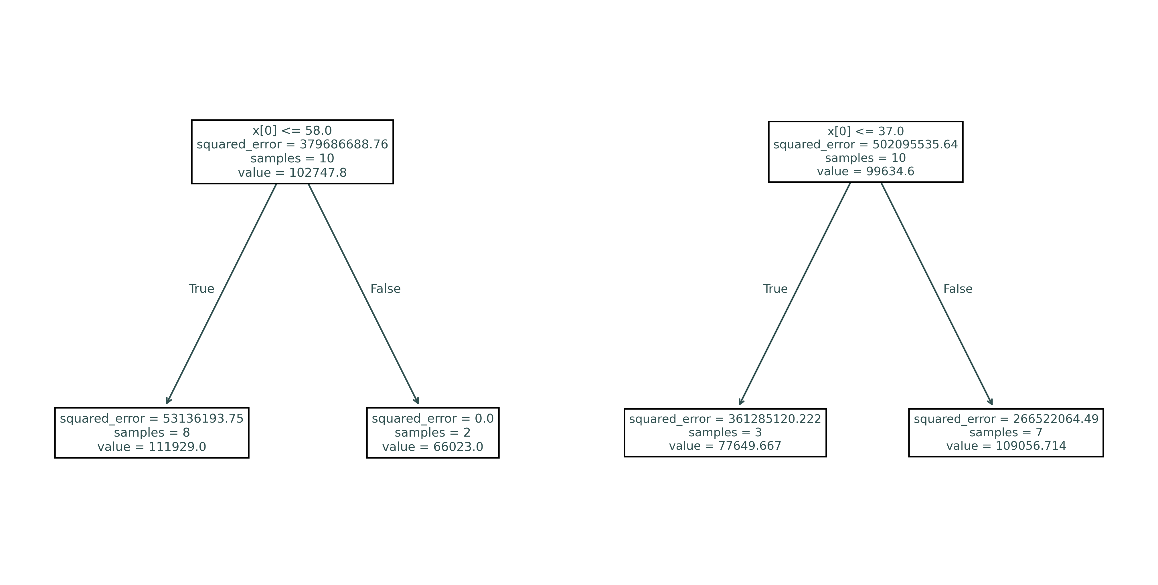
plt.show()Here we see two trees, both fit to a bootstrap resample of some original data, using one split of a randomly chosen feature. Notice that these tress will not make the same predictions.
print(export_text(random_tree_01))|--- feature_0 <= 58.00
| |--- value: [111929.00]
|--- feature_0 > 58.00
| |--- value: [66023.00]
print(export_text(random_tree_02))|--- feature_0 <= 37.00
| |--- value: [77649.67]
|--- feature_0 > 37.00
| |--- value: [109056.71]
Random Forests for Regression
In sklearn, random forests can be used for regression with RandomForestRegressor().
Simulated Sinusoidal Data
To investigate random forests for regression, we will return to the familiar simulated sinusoidal data.
# simulate train data
X_train, y_train = simulate_sin_data(n=200, seed=1)

# simulate test data
X_test, y_test = simulate_sin_data(n=200, seed=2)
tree_default = DecisionTreeRegressor()
_ = tree_default.fit(X_train, y_train)
tree_modified = DecisionTreeRegressor(max_depth=5)
_ = tree_modified.fit(X_train, y_train)
rf_default = RandomForestRegressor()
_ = rf_default.fit(X_train, y_train)
rf_modified = RandomForestRegressor(max_samples=25)
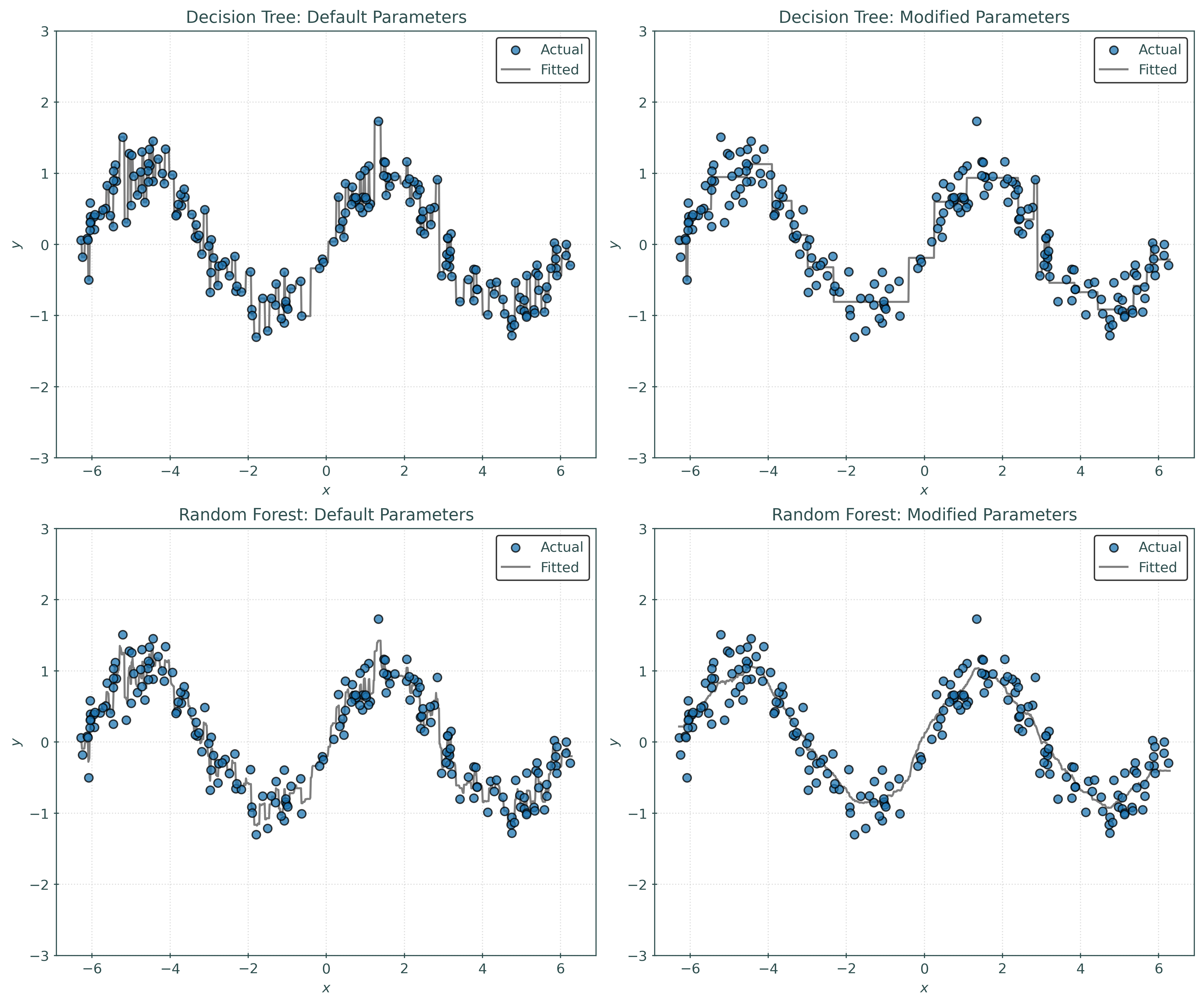
_ = rf_modified.fit(X_train, y_train)We create and fit four models:
- A decision tree with all default parameters.
- A decision tree with some modified parameters.
- A random forest with all default parameters.
- A random forest with some modified parameters.
In this case, we modify the max_samples parameter to the random forest. This parameter is used to control the number of observations in the bootstrap resample. While generally not considered one of the key tuning parameters of a random forest, it can often provide a useful performance benefits. In some sense, decreasing the value of provides an implicit form of regularization.
fig, axs = plt.subplots(2, 2, figsize=(12, 10))

plot_sin_regression(
    tree_default,
    X_train,
    y_train,
    "Decision Tree: Default Parameters",
    ax=axs[0, 0],
)
plot_sin_regression(
    tree_modified,
    X_train,
    y_train,
    "Decision Tree: Modified Parameters",
    ax=axs[0, 1],
)
plot_sin_regression(
    rf_default,
    X_train,
    y_train,
    "Random Forest: Default Parameters",
    ax=axs[1, 0],
)
plot_sin_regression(
    rf_modified,
    X_train,
    y_train,
    "Random Forest: Modified Parameters",
    ax=axs[1, 1],
)

plt.show()
Notice:
- The default tree is obviously overfit. It is an example of a strong learner. It is making far too many splits.
- The modified tree is not overfit, but just by visual inspection, the predictions are too “discrete” in some sense, that is, not smooth enough.
- The default forest already shows improvement over default tree. It avoids the overfitting of the default tree. Visually, this forest looks a bit better than the modified tree, but may not provide much performance improvement.
- The modified forest looks great! Decreasing the samples used when bootstrapping had a “smoothing” effect on the learned regression.
rsme_tree_default = root_mean_squared_error(
    y_test,
    tree_default.predict(X_test),
)

rsme_tree_modified = root_mean_squared_error(
    y_test,
    tree_modified.predict(X_test),
)

rsme_rf_default = root_mean_squared_error(
    y_test,
    rf_default.predict(X_test),
)

rsme_rf_modified = root_mean_squared_error(
    y_test,
    rf_modified.predict(X_test),
)print(f"Test RMSE for default Tree: {rsme_tree_default:.2f}")
print(f"Test RMSE for modified Tree: {rsme_tree_modified:.2f}")
print(f"Test RMSE for default Random Forest: {rsme_rf_default:.2f}")
print(f"Test RMSE for modified Random Forest: {rsme_rf_modified:.2f}")Test RMSE for default Tree: 0.39
Test RMSE for modified Tree: 0.33
Test RMSE for default Random Forest: 0.33
Test RMSE for modified Random Forest: 0.29We see that the test RMSE of each model confirms our visual intuition above.
Simulated Multiple Feature Data
To further investigate random forests, we’ll simulate data using the make_regression from sklearn. The sinusoidal data only contained a single feature, so could not fully showcase the potential of random forests, as they could not use random features during splitting.
# simulate some data for regression
X, y = make_regression(
    n_samples=300,
    n_features=5,
    noise=0.3,
    random_state=42,
)

# train-test split the data
X_train, X_test, y_train, y_test = train_test_split(
    X,
    y,
    test_size=0.25,
    random_state=42,
)
dt2 = DecisionTreeRegressor(max_depth=2)
dt5 = DecisionTreeRegressor(max_depth=5)
rf = RandomForestRegressor()_ = dt2.fit(X_train, y_train)
_ = dt5.fit(X_train, y_train)
_ = rf.fit(X_train, y_train)dt2_pred = dt2.predict(X_test)
dt5_pred = dt5.predict(X_test)
rf_pred = rf.predict(X_test)# setup figure
fig, (ax1, ax2, ax3) = plt.subplots(1, 3, figsize=(15, 5))
# add overall title
fig.suptitle("Predicted versus Actual")
# create subplot for dt
ax1.set_title("Decision Tree: Max Depth 2")
ax1.scatter(y_test, dt2_pred, color="dodgerblue")
ax1.set_xlabel("Actual")
ax1.set_ylabel("Predicted")
ax1.grid(True, linestyle="--", color="lightgrey")
ax1.axline((0, 0), slope=1, color="black")
# create subplot for dt
ax2.set_title("Decision Tree: Max Depth 5")
ax2.scatter(y_test, dt5_pred, color="dodgerblue")
ax2.set_xlabel("Actual")
ax2.set_ylabel("Predicted")
ax2.grid(True, linestyle="--", color="lightgrey")
ax2.axline((0, 0), slope=1, color="black")
# create subplot for rf
ax3.set_title("Random Forest")
ax3.scatter(y_test, rf_pred, color="dodgerblue")
ax3.set_xlabel("Actual")
ax3.set_ylabel("Predicted")
ax3.grid(True, linestyle="--", color="lightgrey")
ax3.axline((0, 0), slope=1, color="black")
# shot plot
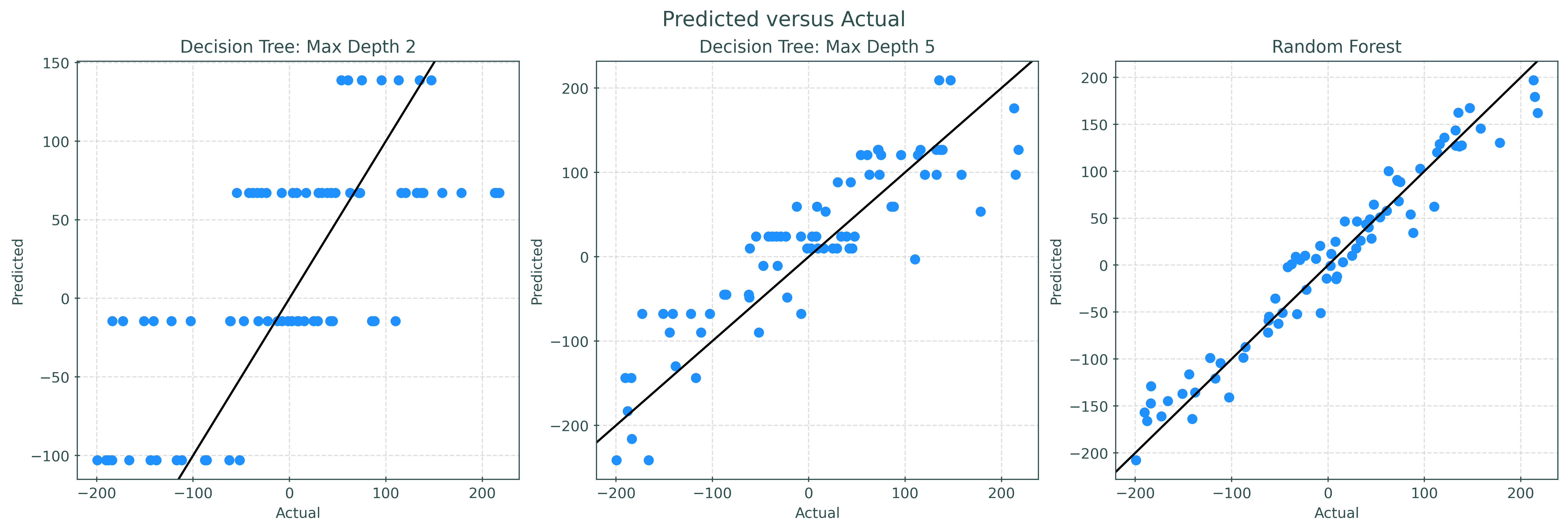
plt.show()Simply looking at the predicted versus actual plots, we can clearly see the random forest outperforming the single trees. (Calculate test RMSE for each to verify!) Also note that with limited depth, trees will only predict a finite number of unique values. Because of the averaging and randomness of random forests, predictions are much less discrete.
Random Forests for Classification
In sklearn, random forests can be used for classification with RandomForestClassifier().
# simulate some data for classification
X, y = make_blobs(
    n_samples=400,
    cluster_std=3,
    random_state=42,
)

# train-test split the data
X_train, X_test, y_train, y_test = train_test_split(
    X,
    y,
    test_size=0.50,
    random_state=42,
)
# create and fit a single decision tree
tree = DecisionTreeClassifier()
_ = tree.fit(X_train, y_train)
# create and fit a random forest
rf = RandomForestClassifier()
_ = rf.fit(X_train, y_train)# calculate test accuracies
acc_tree = accuracy_score(y_test, tree.predict(X_test))
acc_rf = accuracy_score(y_test, rf.predict(X_test))print(f"Test Accuracy for Decision Tree: {acc_tree:.2f}")
print(f"Test Accuracy for Random Forest: {acc_rf:.2f}")Test Accuracy for Decision Tree: 0.97
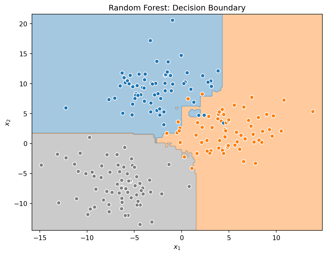
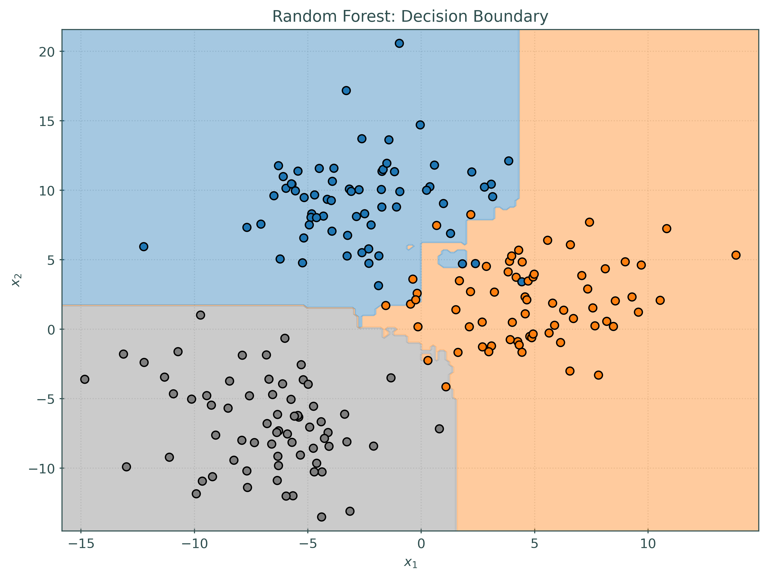
Test Accuracy for Random Forest: 0.95Note that in this (simple) case, the tree actually outperforms the forest! This is certainly possible in practice, but notice that the difference is small, and with more meaningful and complicated data, a random forest will usually outperform a tree. But this should be a reminder that you have to try many models and see what works best! You might also notice that the decision boundaries for the random forest seem more “correct” in the sense that we would doubt that the boundaries can be well represented by simple binary partitions.
tree.predict_proba(X_test[:10])array([[0., 1., 0.],
[1., 0., 0.],
[0., 0., 1.],
[1., 0., 0.],
[0., 1., 0.],
[0., 1., 0.],
[1., 0., 0.],
[1., 0., 0.],
[0., 0., 1.],
[0., 1., 0.]])rf.predict_proba(X_test[:10])array([[0.01, 0.95, 0.04],
[1. , 0. , 0. ],
[0. , 0. , 1. ],
[0.95, 0.05, 0. ],
[0. , 1. , 0. ],
[0.24, 0.76, 0. ],
[1. , 0. , 0. ],
[1. , 0. , 0. ],
[0. , 0. , 1. ],
[0. , 0.96, 0.04]])As always, we can obtain predicted probabilities with a random forest. Note that unlike the tree, these probabilities seem more reasonable and do not simply place a probability of 1 on a class for each observation.
Random forests use the soft voting mechanism to determine probabilities, and thus predictions.
Tuning
To demonstrate tuning with random forests, we will use the diabetes data from sklearn.
# load diabetes data from sklearn
diabetes = load_diabetes(as_frame=True, scaled=False).frame

# train-test split the data
diabetes_train, diabetes_test = train_test_split(
    diabetes,
    test_size=0.2,
    random_state=42,
)

# create the X and y version of the train data
X_train = diabetes_train.drop("target", axis=1)
y_train = diabetes_train["target"]

# create the X and y version of the test data
X_test = diabetes_test.drop("target", axis=1)
y_test = diabetes_test["target"]

# check shapes of data
X_train.shape, y_train.shape, X_test.shape, y_test.shape
((353, 10), (353,), (89, 10), (89,))X_train.head()| age | sex | bmi | bp | s1 | s2 | s3 | s4 | s5 | s6 | |
|---|---|---|---|---|---|---|---|---|---|---|
| 17 | 68.00 | 2.00 | 27.50 | 111.00 | 214.00 | 147.00 | 39.00 | 5.00 | 4.94 | 91.00 |
| 66 | 46.00 | 2.00 | 24.70 | 85.00 | 174.00 | 123.20 | 30.00 | 6.00 | 4.64 | 96.00 |
| 137 | 50.00 | 1.00 | 31.00 | 123.00 | 178.00 | 105.00 | 48.00 | 4.00 | 4.83 | 88.00 |
| 245 | 41.00 | 1.00 | 23.10 | 86.00 | 148.00 | 78.00 | 58.00 | 3.00 | 4.09 | 60.00 |
| 31 | 42.00 | 1.00 | 20.30 | 71.00 | 161.00 | 81.20 | 66.00 | 2.00 | 4.23 | 81.00 |
y_train17 144.00
66 150.00
137 280.00
245 125.00
31 59.00
...
106 134.00
270 202.00
348 148.00
435 64.00
102 302.00
Name: target, Length: 353, dtype: float64# create pipeline
pipeline = Pipeline(
steps=[
(
"regressor",
RandomForestRegressor(random_state=42),
),
]
)In this case we are using a pipeline, but foregoing any preprocessing. Of course, if needed, a ColumnTransformer could be added to this pipeline to preprocess columns. In this case, we have no categorical features, no missing data, and because a random forests uses decision trees, scaling the numeric features is not necessary.
RandomForestRegressor().get_params(){'bootstrap': True,
'ccp_alpha': 0.0,
'criterion': 'squared_error',
'max_depth': None,
'max_features': 1.0,
'max_leaf_nodes': None,
'max_samples': None,
'min_impurity_decrease': 0.0,
'min_samples_leaf': 1,
'min_samples_split': 2,
'min_weight_fraction_leaf': 0.0,
'monotonic_cst': None,
'n_estimators': 100,
'n_jobs': None,
'oob_score': False,
'random_state': None,
'verbose': 0,
'warm_start': False}# define parameter grid
param_grid = {
"regressor__max_features": [1, 3, 10],
"regressor__n_estimators": [25, 100],
"regressor__max_samples": [10, None],
}Here we consider a somewhat simple grid, using only a small subset of possible tuning parameters. In general, max_features and n_estimators will be the most useful parameters to tune. The n_estimators parameter controls the number of trees in the ensemble, while max_features controls the number of random features considered during each split.
For max_features, 3 is approximately the square root of the number of features, which is recommended. Consider also including 1, and the number of features, which here is 10. Using more values than this is likely to give little if any benefit, but be computationally expensive.
Even though we demonstrate tuning here, it is reasonable to simply use a random forest with all default parameters and no tuning.
A nice feature of random forests is their near inability to overfit, another reason why tuning is not high priority for random forests.
# setup grid search with cross-validation
tuned_model = GridSearchCV(
    pipeline,
    param_grid,
    cv=5,
    scoring="neg_root_mean_squared_error",
    verbose=1,
)
# perform grid search with cross-validation
with parallel_backend("loky"):
tuned_model.fit(X_train, y_train)Fitting 5 folds for each of 12 candidates, totalling 60 fitstuned_model.best_estimator_Pipeline(steps=[('regressor',
RandomForestRegressor(max_features=3, random_state=42))])In a Jupyter environment, please rerun this cell to show the HTML representation or trust the notebook. On GitHub, the HTML representation is unable to render, please try loading this page with nbviewer.org.
Pipeline(steps=[('regressor',
RandomForestRegressor(max_features=3, random_state=42))])RandomForestRegressor(max_features=3, random_state=42)
tuned_model.best_params_{'regressor__max_features': 3,
'regressor__max_samples': None,
'regressor__n_estimators': 100}Notice that despite our tuning, we selected the default value for each parameter except for max_samples! And for max_samples, we selected a recommended value.
print(f"Best Model, CV RMSE: {-tuned_model.best_score_:.2f}")Best Model, CV RMSE: 58.41cv_results_to_df(tuned_model.cv_results_).style.hide(axis="index")| max_features | max_samples | n_estimators | mean_test_score | std_test_score |
|---|---|---|---|---|
| 1 | 10.000000 | 25 | -65.27 | 6.05 |
| 1 | 10.000000 | 100 | -64.26 | 5.40 |
| 1 | nan | 25 | -59.69 | 2.90 |
| 1 | nan | 100 | -59.04 | 3.17 |
| 3 | 10.000000 | 25 | -63.48 | 5.02 |
| 3 | 10.000000 | 100 | -62.17 | 4.62 |
| 3 | nan | 25 | -59.56 | 3.49 |
| 3 | nan | 100 | -58.41 | 4.37 |
| 10 | 10.000000 | 25 | -60.57 | 4.21 |
| 10 | 10.000000 | 100 | -59.67 | 4.08 |
| 10 | nan | 25 | -59.61 | 4.88 |
| 10 | nan | 100 | -59.11 | 4.87 |
Note that for the same max_samples and n_estimators, the max_features parameter does not have a large effect. It seems that limiting max_samples has a negative effect, and n_estimators does note make a huge difference.
Note that a downside of random forests is their large “size” when serializing. Reducing n_estimators can reduce the model size, but can often come with a performance tradeoff.
print(f"Test RMSE: {-tuned_model.score(X_test, y_test):.2f}")Test RMSE: 53.18Notice that the test RMSE here is significantly lower than the cross-validated results. In this case, we suspect this is due to the trees being fit to less data during cross-validation. This is consistent with our findings related to the max_samples parameter.
Alternatives to Grid Search and Cross-Validation
With big data, performing cross-validation for a random forest, especially with a grid search, can become computationally expensive.
As an alternative, random forests can use “out of bag” estimates.
Consider using these in practice. In CS 307, we will prefer a cross-validated grid search for consistency.
Boosting
While bagging considers the average of many strong learners fit in parallel, boosting uses many weak learners in sequence.
We will not investigate the details of boosting as thoroughly as random forests. Instead, we will focus on their practical usage.
In general, boosted models train a sequence of weak learners, where each learner is designed to address the shortcomings (errors or misclassifications) of the previous learner. Initially, all training samples are given equal weight. After each iteration, the weights of samples with higher “errors” are increased, so subsequent learners focus more on those “difficult” cases. This sequential process continues until a specified number of learners are trained or the model achieves a desired level of performance.
Unlike random forests, which can often be trained without much consideration to tuning, boosting is much more sensitive to its tuning parameters. In particular, care should be given to the number of iterations (learners) considered.
Boosted models have a reputation for winning Kaggle competitions, usually through a combination of clever feature engineering, appropriate preprocessing, and detailed tuning.
Boosting has many variants. Some popular modern variants include:
From some, an sklearn API is available, but none are implemented directly in sklearn.
Within sklearn, two more classic boosting techniques are available:
- AdaBoost
- Regression:
sklearn.ensemble.AdaBoostRegressor - Classification:
sklearn.ensemble.AdaBoostClassifier|sklearnAPI
- Regression:
- Gradient Boosting
- Regression:
sklearn.ensemble.GradientBoostingRegressor - Classification:
sklearn.ensemble.GradientBoostingClassifier|sklearnAPI
- Regression:
Despite these available choices, we will recommend the use of Histogram Gradient Boosting Trees, which is an sklearn model that is inspired by LightGBM. It combines the best of the sklearn interface with the speed and performance of LightGBM.
Histogram Gradient Boosting Regression Trees
Simulated Sinusoidal Data
# simulate train data
X_train, y_train = simulate_sin_data(n=200, seed=1)

# simulate test data
X_test, y_test = simulate_sin_data(n=200, seed=2)
tree_default = DecisionTreeRegressor()
_ = tree_default.fit(X_train, y_train)
tree_modified = DecisionTreeRegressor(max_depth=5)
_ = tree_modified.fit(X_train, y_train)
hb_default = HistGradientBoostingRegressor()
_ = hb_default.fit(X_train, y_train)
hb_modified = HistGradientBoostingRegressor(learning_rate=0.01)
_ = hb_modified.fit(X_train, y_train)fig, axs = plt.subplots(2, 2, figsize=(12, 10))
plot_sin_regression(
tree_default,
X_train,
y_train,
"Decision Tree: Default Parameters",
ax=axs[0, 0],
)
plot_sin_regression(
tree_modified,
X_train,
y_train,
"Decision Tree: Modified Parameters",
ax=axs[0, 1],
)
plot_sin_regression(
hb_default,
X_train,
y_train,
"Boosting: Default Parameters",
ax=axs[1, 0],
)
plot_sin_regression(
hb_modified,
X_train,
y_train,
"Boosting: Modified Parameters",
ax=axs[1, 1],
)
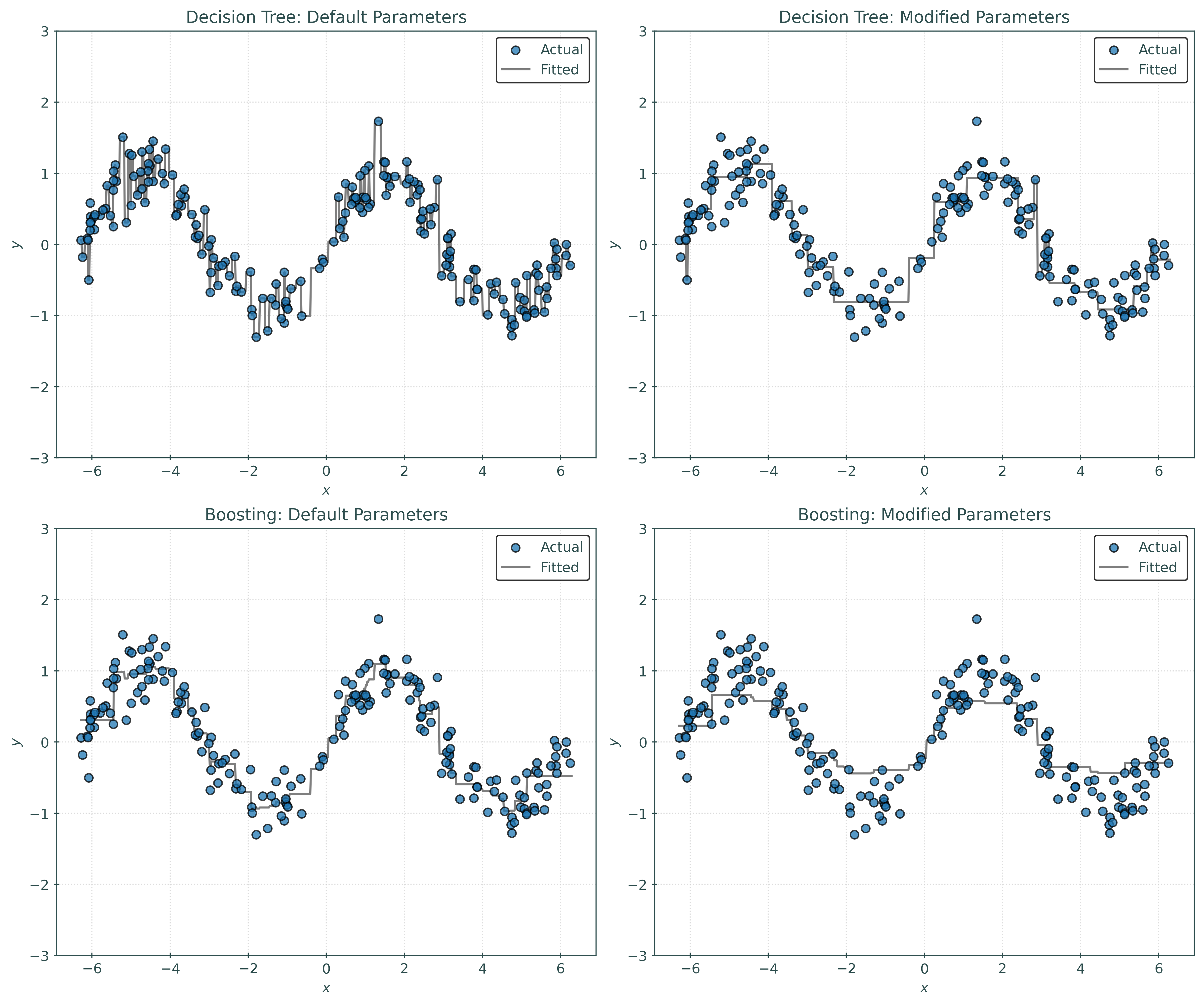
plt.show()Here we see similar results as we did with the random forest. The default boosted model works quite well! The non-default boosted model uses a lower learning rate, and from this plot alone, we can clearly see that it “learned” less.
rsme_tree_default = root_mean_squared_error(
    y_test,
    tree_default.predict(X_test),
)

rsme_tree_modified = root_mean_squared_error(
    y_test,
    tree_modified.predict(X_test),
)

rsme_hb_default = root_mean_squared_error(
    y_test,
    hb_default.predict(X_test),
)

rsme_hb_modified = root_mean_squared_error(
    y_test,
    hb_modified.predict(X_test),
)print(f"Test RMSE for default Tree: {rsme_tree_default:.2f}")
print(f"Test RMSE for modified Tree: {rsme_tree_modified:.2f}")
print(f"Test RMSE for default Boosting: {rsme_hb_default:.2f}")
print(f"Test RMSE for modified Boosting: {rsme_hb_modified:.2f}")Test RMSE for default Tree: 0.39
Test RMSE for modified Tree: 0.33
Test RMSE for default Boosting: 0.31
Test RMSE for modified Boosting: 0.42Again, the test metrics match our intuition, with the default boosted model working quite well!
Simulated Multiple Feature Data
# simulate some data for regression
X, y = make_regression(
    n_samples=300,
    n_features=5,
    noise=0.3,
    random_state=42,
)

# train-test split the data
X_train, X_test, y_train, y_test = train_test_split(
    X,
    y,
    test_size=0.25,
    random_state=42,
)
dt2 = DecisionTreeRegressor(max_depth=2)
dt5 = DecisionTreeRegressor(max_depth=5)
hb = HistGradientBoostingRegressor()_ = dt2.fit(X_train, y_train)
_ = dt5.fit(X_train, y_train)
_ = hb.fit(X_train, y_train)dt2_pred = dt2.predict(X_test)
dt5_pred = dt5.predict(X_test)
hb_pred = hb.predict(X_test)# setup figure
fig, (ax1, ax2, ax3) = plt.subplots(1, 3)
fig.set_size_inches(16, 5)
fig.set_dpi(100)
# add overall title
fig.suptitle("Predicted versus Actual")
# create subplot for dt
ax1.set_title("Decision Tree: Max Depth 2")
ax1.scatter(y_test, dt2_pred, color="dodgerblue")
ax1.set_xlabel("Actual")
ax1.set_ylabel("Predicted")
ax1.grid(True, linestyle="--", color="lightgrey")
ax1.axline((0, 0), slope=1, color="black")
# create subplot for dt
ax2.set_title("Decision Tree: Max Depth 5")
ax2.scatter(y_test, dt5_pred, color="dodgerblue")
ax2.set_xlabel("Actual")
ax2.set_ylabel("Predicted")
ax2.grid(True, linestyle="--", color="lightgrey")
ax2.axline((0, 0), slope=1, color="black")
# create subplot for rf
ax3.set_title("Boosting")
ax3.scatter(y_test, hb_pred, color="dodgerblue")
ax3.set_xlabel("Actual")
ax3.set_ylabel("Predicted")
ax3.grid(True, linestyle="--", color="lightgrey")
ax3.axline((0, 0), slope=1, color="black")
# shot plot
plt.show()Much like we saw with random forests, the histogram gradient boosting trees clearly outperform the individual trees. (Again, you should calculate the test RMSE for each to verify!)
Histogram Gradient Boosting Classification Trees
# simulate some data for classification
X, y = make_blobs(
    n_samples=400,
    cluster_std=3,
    random_state=42,
)

# train-test split the data
X_train, X_test, y_train, y_test = train_test_split(
    X,
    y,
    test_size=0.50,
    random_state=42,
)
# create and fit a single decision tree
tree = DecisionTreeClassifier()
_ = tree.fit(X_train, y_train)
# create and fit a boosted model
hb = HistGradientBoostingClassifier()
_ = hb.fit(X_train, y_train)# calculate test accuracies
acc_tree = accuracy_score(y_test, tree.predict(X_test))
acc_hb = accuracy_score(y_test, hb.predict(X_test))print(f"Test Accuracy for Decision Tree: {acc_tree:.2f}")
print(f"Test Accuracy for Boosted Trees: {acc_rf:.2f}")Test Accuracy for Decision Tree: 0.97
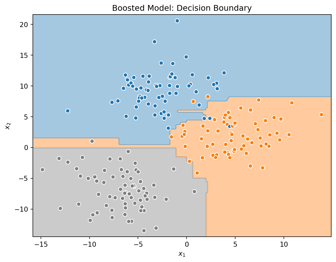
Test Accuracy for Boosted Trees: 0.95Again, in this (simple) case, the tree actually outperforms the ensemble!
tree.predict_proba(X_test[:10])array([[0., 1., 0.],
[1., 0., 0.],
[0., 0., 1.],
[1., 0., 0.],
[0., 1., 0.],
[0., 1., 0.],
[1., 0., 0.],
[1., 0., 0.],
[0., 0., 1.],
[0., 1., 0.]])np.round(hb.predict_proba(X_test[:10]), 4)array([[0. , 1. , 0. ],
[1. , 0. , 0. ],
[0. , 0. , 1. ],
[1. , 0. , 0. ],
[0. , 1. , 0. ],
[0.0052, 0.9948, 0. ],
[1. , 0. , 0. ],
[1. , 0. , 0. ],
[0. , 0. , 1. ],
[0. , 1. , 0. ]])As always, we can obtain predicted probabilities. The predicted probabilities for the boosted tree seem slightly more reasonable than the tree, but not quite as nice as the random forest we saw previously.
Tuning
To demonstrate tuning with HGBT, we will use the breast cancer data from sklearn.
# load cancer data from sklearn
cancer = load_breast_cancer(as_frame=True).frame

# train-test split the data
cancer_train, cancer_test = train_test_split(
    cancer,
    test_size=0.2,
    random_state=42,
)

# create the X and y version of the train data
X_train = cancer_train.iloc[:, :10]
y_train = cancer_train["target"]

# create the X and y version of the test data
X_test = cancer_test.iloc[:, :10]
y_test = cancer_test["target"]

# check shapes of data
X_train.shape, y_train.shape, X_test.shape, y_test.shape
((455, 10), (455,), (114, 10), (114,))For simplicity, we consider only the first 10 features.
X_train.head()| mean radius | mean texture | mean perimeter | mean area | mean smoothness | mean compactness | mean concavity | mean concave points | mean symmetry | mean fractal dimension | |
|---|---|---|---|---|---|---|---|---|---|---|
| 68 | 9.03 | 17.33 | 58.79 | 250.50 | 0.11 | 0.14 | 0.31 | 0.04 | 0.21 | 0.08 |
| 181 | 21.09 | 26.57 | 142.70 | 1,311.00 | 0.11 | 0.28 | 0.25 | 0.15 | 0.24 | 0.07 |
| 63 | 9.17 | 13.86 | 59.20 | 260.90 | 0.08 | 0.09 | 0.06 | 0.02 | 0.23 | 0.07 |
| 248 | 10.65 | 25.22 | 68.01 | 347.00 | 0.10 | 0.07 | 0.02 | 0.02 | 0.19 | 0.06 |
| 60 | 10.17 | 14.88 | 64.55 | 311.90 | 0.11 | 0.08 | 0.01 | 0.01 | 0.27 | 0.07 |
y_train68 1
181 0
63 1
248 1
60 1
..
71 1
106 1
270 1
435 0
102 1
Name: target, Length: 455, dtype: int64# create pipeline
pipeline = Pipeline(
steps=[
(
"classifier",
HistGradientBoostingClassifier(random_state=42),
),
]
)Here we create a pipeline, mostly for consistency. We do not perform any preprocessing, but a ColumnTransformer could be added there were a need to add preprocessing like handling of missing data.
HistGradientBoostingClassifier().get_params(){'categorical_features': 'warn',
'class_weight': None,
'early_stopping': 'auto',
'interaction_cst': None,
'l2_regularization': 0.0,
'learning_rate': 0.1,
'loss': 'log_loss',
'max_bins': 255,
'max_depth': None,
'max_features': 1.0,
'max_iter': 100,
'max_leaf_nodes': 31,
'min_samples_leaf': 20,
'monotonic_cst': None,
'n_iter_no_change': 10,
'random_state': None,
'scoring': 'loss',
'tol': 1e-07,
'validation_fraction': 0.1,
'verbose': 0,
'warm_start': False}# define parameter grid
param_grid = {
"classifier__learning_rate": [0.1, 0.25],
"classifier__max_iter": [100, 200],
"classifier__max_features": [0.25, 0.5, 1.0],
}Here we consider a somewhat simple grid, using only a small subset of possible tuning parameters. In general, learning_rate and max_iter will be the most useful parameters to tune. The learning rate should be greater than 0 and at most 1. Think of the learning rate as controlling how much each base learner can learn. The max_iter parameter controls the number of learners to use. This parameter needs special attention, as setting it too high can cause overfitting.
Be careful: Specifying a large grid will lead to long tuning times!
# setup grid search with cross-validation
tuned_model = GridSearchCV(
    pipeline,
    param_grid,
    cv=5,
    scoring="accuracy",
    verbose=1,
)
# perform grid search with cross-validation
with parallel_backend("loky"):
tuned_model.fit(X_train, y_train)Fitting 5 folds for each of 12 candidates, totalling 60 fitstuned_model.best_estimator_Pipeline(steps=[('classifier',
HistGradientBoostingClassifier(max_features=0.5, max_iter=200,
random_state=42))])In a Jupyter environment, please rerun this cell to show the HTML representation or trust the notebook. On GitHub, the HTML representation is unable to render, please try loading this page with nbviewer.org.
Pipeline(steps=[('classifier',
                 HistGradientBoostingClassifier(max_features=0.5, max_iter=200,
random_state=42))])HistGradientBoostingClassifier(max_features=0.5, max_iter=200, random_state=42)
tuned_model.best_params_{'classifier__learning_rate': 0.1,
'classifier__max_features': 0.5,
'classifier__max_iter': 200}cv_results_to_df(tuned_model.cv_results_).style.hide(axis="index")| learning_rate | max_features | max_iter | mean_test_score | std_test_score |
|---|---|---|---|---|
| 0.100000 | 0.250000 | 100 | 0.95 | 0.02 |
| 0.100000 | 0.250000 | 200 | 0.94 | 0.02 |
| 0.100000 | 0.500000 | 100 | 0.95 | 0.02 |
| 0.100000 | 0.500000 | 200 | 0.95 | 0.01 |
| 0.100000 | 1.000000 | 100 | 0.95 | 0.02 |
| 0.100000 | 1.000000 | 200 | 0.95 | 0.02 |
| 0.250000 | 0.250000 | 100 | 0.95 | 0.02 |
| 0.250000 | 0.250000 | 200 | 0.95 | 0.02 |
| 0.250000 | 0.500000 | 100 | 0.95 | 0.02 |
| 0.250000 | 0.500000 | 200 | 0.94 | 0.01 |
| 0.250000 | 1.000000 | 100 | 0.94 | 0.03 |
| 0.250000 | 1.000000 | 200 | 0.94 | 0.03 |
Here, we actually see very little effect of tuning, but that is due to the simplicity of the data. In practice, tuning will have a greater effect.
print(f"Best Model, CV Accuracy: {tuned_model.best_score_:.2f}")Best Model, CV Accuracy: 0.95print(f"Test Accuracy: {tuned_model.score(X_test, y_test):.2f}")Test Accuracy: 0.96np.round(tuned_model.predict_proba(X_test[:10]), 3)array([[0. , 1. ],
[1. , 0. ],
[1. , 0. ],
[0. , 1. ],
[0. , 1. ],
[1. , 0. ],
[1. , 0. ],
[0.481, 0.519],
[0.247, 0.753],
[0. , 1. ]])Alternatives to Grid Search and Cross-Validation
With big data, and a decent sized grid, performing cross-validation together with a grid search can become computationally expensive.
As an alternative, histogram gradient boosting trees in sklearn have parameters for early stopping (early_stopping) and validation sets (validation_fraction). Consider using these in practice. In CS 307, we will prefer a cross-validated grid search for consistency.
Additionally, rather than an exhaustive grid search, a randomized search can be used. By randomly sampling from the parameter space, a randomized search can be much faster than a grid search.
Additional Resources
For more information on the details and usage of boosting, consider the following video series:
Summary and Comparison
- Random Forests are an ensemble of strong learners in parallel.
- Random forests do not require much tuning, as they are hard to overfit.
- Boosted Models are an ensemble of weak learners in sequence.
- Boosting is sensitive to tuning, and can overfit.
Miscellaneous
A related method called stacking is another form of an ensemble method that includes a meta-learner on top of the base learners.
